Update. The GitHub repository now contains several additional examples besides the code discussed in this article.
This is the third and probably final practical article in a series on variational auto-encoders and their implementation in Torch. Based on the Gaussian variational auto-encoder [] implemented in a previous article, this article discusses a simple implementation of a Bernoulli variational auto-encoder [][] where the latent variables are assumed to be Bernoulli distributed.
Previous articles:
- The Mathematics of Variational Auto-Encoders
- Denoising Variational Auto-Encoders
- Categorical Variational Auto-Encoders
- Variational Auto-Encoder in Torch
- Denoising Variational Auto-Encoder in Torch
Prerequisites. This article requires basic understanding of LUA and Torch; the code is also based on this article and the underlying mathematics are detailed in this article.
The code is available on GitHub:
Torch Denoising Variational Auto-Encoder on GitHubOverview
The original variational auto-encoder as in [] is a continuous latent variable model. The model is intended to learn a latent space $\mathcal{Z} = \mathbb{R}^Q$ using a given set of samples $\{y_m\} \subseteq \mathcal{Y} = \mathbb{R}^R$ where $Q \ll R$. The model consists of the generative model $p(y | z)$ given a fixed prior $p(z)$, and the recognition (inference) model $q(z | y)$. The vanilla variational auto-encoder imposes a unit Gaussian prior
$p(z) = \mathcal{N}(z; 0, I_Q)$
such that the recognition model $q(z | y)$ also needs to be modeled as Gaussian distribution. The corresponding loss to be minimized can be written as:
$\mathcal{L}_{\text{VAE}} (w) = \text{KL}(q(z|y_m) | p(z)) - \frac{1}{L}\sum_{l = 1}^L \ln p(y_m | z_{l,m})$
where $y_m$ is a training sample and $z_{l,m} = g(\epsilon_{l,m}, y)$ with $\epsilon_{l,m} \sim \mathcal{N}(\epsilon ; 0, I_Q)$. Here, $g$ represents the so-called reparamterization trick:
$z_i = g_i(y, \epsilon_i) = \mu_i(y) + \epsilon_i \sigma_i^2(y)$
which ensures the differentiability of the model with respect to its input.
The latent variables can, however, also be modeled as discrete distributions. For example, the prior $p(z)$ and the recognition model $q(z|y)$ can both be modeled using Bernoulli distributions:
$p(z) = \prod_{i = 1}^Q \text{Ber}(z_i; 0.5)$
$q(z|x) = \prod_{i = 1}^Q \text{Ber}(z_i; \theta_i(y))$
where $\theta_i(y)$ is predicted by the encoder. The main difficulty of this latent space model is the reparameterization trick that allows to sample from $q(z|x)$ in a differentiable manner. In [][], this problem was solved using the following reparameterization trick, which has to be followed by a Sigmoid activation:
$z_i = g(y, \epsilon) = \sigma\left(\ln \epsilon - \ln (1 - \epsilon) + \ln \theta_i(y) - \ln (1 - \theta_i(y))\right)$(1)
where $\epsilon \sim U(0,1)$ is a uniformly distributed auxiliary variable. Finally, the loss to be minimized is, again,
$\mathcal{L}_{\text{VAE}} (w) = \text{KL}(q(z|y_m) | p(z)) - \frac{1}{L}\sum_{l = 1}^L \ln p(y_m | z_{l,m})$
where the Kullback-Leibler divergence is computed analytically as
$\text{KL}(q(z_i | y) | p(z_i)) = \text{KL}(\text{Ber}(z_i; \theta_i(y)) | \text{Ber}(z_i; 0.5))$
$=\sum_{k \in \{0,1\}} \ln \theta_i(y)^k (1 - \theta_i(y))^{1 - k} - \ln 0.5^k 0.5^{1-k}$.(2)
Implementation
The full implementation is discussed below.
-- Bernoulli variational auto-encoder.

require('math')
require('torch')
require('nn')
require('cunn')
require('optim')
require('image')

-- (1) The Kullback Leiber loss follows the Kullback Leibler loss of the Gaussian VAE.
-- The Kullback-Leibler divergence between two Bernoulli distribution can easily
-- be written down by summing over all possible states (i.e. 0 and 1).
--- @class KullbackLeiberDivergence
local KullbackLeiberDivergence, KullbackLeiberDivergenceParent = torch.class('nn.KullbackLeiberDivergence', 'nn.Module')

--- Initialize.
-- @param lambda weight of loss
function KullbackLeiberDivergence:__init(lambda, sizeAverage)
  self.lambda = lambda or 1
  self.prior = 0.5
  self.sizeAverage = sizeAverage or false
  self.loss = 0
end

--- Compute the Kullback-Leiber divergence; however, the input remains
-- unchanged - the divergence is saved in KullBackLeiblerDivergence.loss.
-- @param input probabilities
-- @return probabilities
function KullbackLeiberDivergence:updateOutput(input)

  -- (1.1) Forward pass of the KL divergence which is essentially
  -- an expectation over the log of the quotient of two Bernoulli distributions.
  -- Thus, considering all possible states (0, 1), this can be computed directly.
  self.loss = torch.cmul(input, torch.log(input + 1e-20) - torch.log(self.prior))
    + torch.cmul(1 - input, torch.log(1 - input + 1e-20) - torch.log(1 - self.prior))
  self.loss = self.lambda*torch.sum(self.loss)

  if self.sizeAverage then
    self.loss = self.loss/lib.utils.storageProd(#input)
  end

  self.output = input
  return self.output
end

--- Compute the backward pass of the Kullback-Leibler Divergence.
-- @param input probabilities
-- @param gradOutput gradients from top layer
-- @return gradients from top layer plus gradient of KL divergence with respect to probabilities
function KullbackLeiberDivergence:updateGradInput(input, gradOutput)

  -- (1.2) Backward pass, i.e. derivative of (1.1).
  local ones = input:clone():fill(1)
  self.gradInput = torch.log(input + 1e-20) + 1 - torch.log(self.prior) - torch.cdiv(ones, 1 - input + 1e-20)
    - torch.log(1 - input + 1e-20) + torch.cdiv(input, 1 - input + 1e-20) + torch.log(1 - self.prior)
  self.gradInput = self.lambda*self.gradInput
  --assert(not torch.any(self.gradInput:ne(self.gradInput)))

  if self.sizeAverage then
    self.gradInput = self.gradInput/lib.utils.storageProd(#input)
  end

  self.gradInput = self.gradInput + gradOutput
  --print(torch.mean(self.gradInput))
  return self.gradInput
end

-- (2) The reparameterization trick assumes that the next layer is a Sigmoid layer
-- in order to function correctly.
--- @class ReparameterizationSampler
local ReparameterizationSampler, ReparameterizationSamplerParent = torch.class('nn.ReparameterizationSampler', 'nn.Module')

--- Initialize.
-- @param temperature temperature of prediction
function ReparameterizationSampler:__init(temperature)
  self.temperature = temperature or 1
end

--- Sample from the provided mean and variance using the reparameterization trick.
-- @param input Bernoulli probabilities
-- @return sample
function ReparameterizationSampler:updateOutput(input)

  -- (2.1) Reparameterization:
  -- Let u be a uniform random variale in [0,1], p be the predicted probability (i.e. input),
  -- let l be the temperature.
  -- y = sigmoid((log(p) + log(u) - log(1 - u))/l)
  self.eps = torch.rand(input:size()):cuda()

  --self.output = (torch.log(input + 1e-20) + torch.log(self.eps) - torch.log(1 - self.eps))/self.temperature
  self.output = (torch.log(input + 1e-20) - torch.log(-torch.log(self.eps + 1e-20) + 1e-20))/self.temperature
  --print(torch.sigmoid(self.output))
  return self.output
end

--- Backward pass of the sampler.
-- @param input Bernoulli probabilities
-- @param gradOutput gradients of top layer
-- @return gradients with respect to input, table of two elements
function ReparameterizationSampler:updateGradInput(input, gradOutput)

  -- (2.2) Derivative of reparameterization with respect to p.
  --local ones = input:clone():fill(1)
  --self.gradInput = torch.cmul(torch.cdiv(ones, input*self.temperature + 1e-20), gradOutput)
  self.gradInput = torch.cdiv(gradOutput, input + 1e-20)/self.temperature
  --assert(not torch.any(self.gradInput:ne(self.gradInput)))
  --print(torch.mean(self.gradInput))
  return self.gradInput
end

-- Data parameters.
H = 24
W = 24
rH = 8
rW = 8
N = 50000

-- Fix random seed.
torch.manualSeed(1)

inputs = torch.Tensor(N, 1, H, W):fill(0)
for i = 1, N do
  local h = torch.random(rH, rH)
  local w = torch.random(rW, rW)
  local aH = torch.random(1, H - h)
  local aW = torch.random(1, W - w)
  inputs[i][1]:sub(aH, aH + h, aW, aW + w):fill(1)
end

outputs = inputs:clone()

-- (3) The encoder consists of several linear layerReparameterizationSamplers followed by
-- the Kullback Leibler loss, the samples and the docoder; the decoder
-- mirrors the encoder.
-- (3.1) The encoder, as for vanilla VAE.
hidden = math.floor(2*H*W)
encoder = nn.Sequential()
encoder:add(nn.View(1*H*W))
encoder:add(nn.Linear(1*H*W, hidden))
--encoder:add(nn.BatchNormalization(hidden))
encoder:add(nn.ReLU(true))
encoder:add(nn.Linear(hidden, hidden))
--encoder:add(nn.BatchNormalization(hidden))
encoder:add(nn.ReLU(true))

code = 25
encoder:add(nn.Linear(hidden, code))

-- (3.2) As for vanilla VAEs.
decoder = nn.Sequential()
decoder:add(nn.Linear(code, hidden))
--decoder:add(nn.BatchNormalization(hidden))
decoder:add(nn.ReLU(true))
decoder:add(nn.Linear(hidden, hidden))
--decoder:add(nn.BatchNormalization(hidden))
decoder:add(nn.ReLU(true))
decoder:add(nn.Linear(hidden, 1*H*W))
decoder:add(nn.View(1, H, W))
decoder:add(nn.Sigmoid(true))

-- (3) The full model, i.e encoder followed by the Kullback Leibler
-- divergence and the reparameterization trick sampler.
-- The main difference to the Gaussian model is that a Sigmoid layer follows
-- the reparameterization sampler.
model = nn.Sequential()
model:add(encoder)
KLD = nn.KullbackLeiberDivergence()
model:add(nn.Sigmoid(true))
model:add(KLD)
model:add(nn.ReparameterizationSampler())
model:add(nn.Sigmoid(true))
model:add(decoder)
print(model)
model = model:cuda()

criterion = nn.BCECriterion()
criterion.sizeAverage = false
criterion = criterion:cuda()

parameters, gradParameters = model:getParameters()
parameters = parameters:cuda()
gradParameters = gradParameters:cuda()

batchSize = 16
learningRate = 0.001
epochs = 10
iterations = epochs*math.floor(N/batchSize)
lossIterations = 50 -- in which interval to report training
protocol = torch.Tensor(iterations, 2):fill(0)

for t = 1, iterations do

  -- Sample a random batch from the dataset.
  local shuffle = torch.randperm(N)
  shuffle = shuffle:narrow(1, 1, batchSize)
  shuffle = shuffle:long()

  local input = inputs:index(1, shuffle)
  local output = outputs:index(1, shuffle)

  input = input:cuda()
  output = output:cuda()

  --- Definition of the objective on the current mini-batch.
  -- This will be the objective fed to the optimization algorithm.
  -- @param x input parameters
  -- @return object value, gradients
  local feval = function(x)

    -- Get new parameters.
    if x ~= parameters then
      parameters:copy(x)
    end

    -- Reset gradients.
    gradParameters:zero()

    -- Evaluate function on mini-batch.
    local pred = model:forward(input)
    local f = criterion:forward(pred, output)

    protocol[t][1] = f
    protocol[t][2] = KLD.loss

    -- Estimate df/dW.
    local df_do = criterion:backward(pred, output)
    model:backward(input, df_do)

    -- return f and df/dX
    return f, gradParameters
  end

  adamState = adamState or {
      learningRate = learningRate,
      momentum = 0,
      learningRateDecay = 5e-7
  }

  -- Returns the new parameters and the objective evaluated
  -- before the update.
  p, f = optim.adam(feval, parameters, adamState)

  if t%lossIterations == 0 then
    local loss = torch.mean(protocol:narrow(2, 1, 1):narrow(1, t - lossIterations + 1, lossIterations))
    local KLDLoss = torch.mean(protocol:narrow(2, 2, 1):narrow(1, t - lossIterations + 1, lossIterations))
    print('[Training] ' .. t .. '/' .. iterations .. ': ' .. loss .. ' | ' .. KLDLoss)
  end
end

randoms = torch.Tensor(20 * H, 20 * W)

-- Sample 20 x 20 points
for i = 1, 20  do
  for j = 1, 20 do
    local sample = torch.rand(1, code)
    sample[sample:gt(0.5)] = 1
    sample[sample:lt(1)] = 0
    local random = decoder:forward(sample:cuda())
    random = random:float()
    randoms[{{(i - 1) * H + 1, i * H}, {(j - 1) * W + 1, j * W}}] = random
  end
end

image.save('random.png', randoms)
The implementation mostly follows our implementation of the original variational auto-encoder, except for some minor changes. Also note that the size of the latent space $\mathcal{Z}$ needs to be increased significantly. While $2$ dimensions were sufficient before, significantly more binary dimensions are needed — which also influences training time.
- The Kullback-Leibler loss can be calculated analytically, as both the prior $p(z_i)$ and the recognition model $q(z_i|x)$ are Bernoulli distributed.
- The forward pass essentially implemented Equation (2).
- In the backward pass, Equation (2) is differentiated with respect to the predicted probabilities $\theta_i(y)$.
- The reparameterization trick which can be found in Equation (1) is also implemented as separate
nnmodule.- In the forward pass, a $\epsilon \sim U(0,1)$ is sampled and Equation (1) is applied. Additionally, the module implements a temperature parameters; the higher the temperature, the closer the approximation comes to true sampling from Bernoulli variables. The implementation also illustrates that a Sigmoid activation module needs to follow the reparameterization module.
- The backward pass implements the derivative of Equation (1) with respect to the sampled variables; which is made possible by the random auxiliary variable $\epsilon$.
- The overall model changes only slightly; specifically, after the encoder, the Kullback-Leibler divergence and the reparameterization layers are added. Finally, a sigmoid activation layer needs to be added before the decoder.
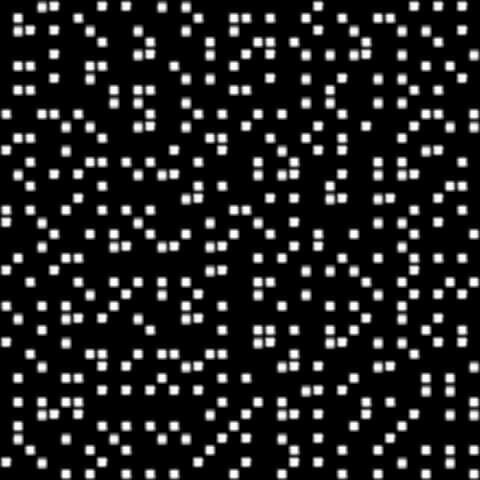
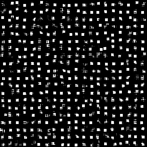
Figure 1 (click to enlarge): Random samples from the learned latent space for a $2$-dimensional space (left) and a $50$-dimensional space (right).
Qualitative results are shown in Figure 1. The results also illustrate the implications of binary latent variables as — for the same dimensionality — expressiveness of the generative model is lost. For a $2$-dimensional latent space, in particular, we see that the model can only capture binary steps in both directions. For a $50$-dimensional latent space, the model is able to interpolate better, but the reconstructions are still inferior to continuous latent variables.
- [] D. P. Kingma and M. Welling. Auto-encoding variational bayes. CoRR, abs/1312.6114, 2013.
- [] D. J. Im, S. Ahn, R. Memisevic, and Y. Bengio. Denoising criterion for variational auto-encoding framework. In AAAI Conference on Artificial Intelligence, pages 2059-2065, 2017.
- [] E. Jang, S. Gu, and B. Poole. Categorical reparameterization with gumbel-softmax. CoRR, abs/1611.01144, 2016.
- [] C. J. Maddison, A. Mnih, and Y. W. Teh. The concrete distribution: A continuous relaxation of discrete random variables. CoRR, abs/1611.00712, 2016.