Update. The GitHub repository now contains several additional examples besides the code discussed in this article.
This is the first practical article in a series on variational auto-encoders []. Before, we discussed the mathematics of variational inference and variational auto-encoders. In this article, we will discuss a Torch implementation of variational auto-encoders.
Previous articles:
- The Mathematics of Variational Auto-Encoders
- Denoising Variational Auto-Encoders
- Categorical Variational Auto-Encoders
Prerequisites. This article requires basic understanding of LUA and Torch; understanding neural networks and optimization will also be helpful. However, as LUA is a simple scripting language, the code should be easy to understand for readers with a background in similar programming languages such as Python. Still, reading this primer might be helpful. This article is based on the mathematical discussion in this article.
The code is available on GitHub:
Torch Variational Auto-Encoder on GitHubOverview
A variational auto-encoder is a continuous latent variable model intended to learn a latent space $\mathcal{Z} = \mathbb{R}^Q$ using a given set of samples $\{y_m\} \subseteq \mathcal{Y} = \mathbb{R}^R$ where $Q \ll R$ (i.e. a dimensionality reduction). The model consists of a decoder — the generative model $p(y | z)$ given a fixed prior $p(z)$ — and an encoder — the recognition model $q(z | y)$. For simplicity, the prior $p(z)$ is modeled as unit Gaussian,
$p(z) = \mathcal{N}(z; 0, I_Q)$,
such that the recognition model $q(z | y)$ is also modeled as Gaussian distribution. Specifically, the encoder predicts the mean and variance, $\mu(y), \sigma^2(z) \in \mathbb{R}^Q$, and the recognition model takes the form
$q(z|y) = \mathcal{N}(z; \mu(y), \text{diag}(\sigma^2(z)))$.
In our example, the training samples $y_m$ will be binary images such that the generative model can be written as follows:
$p(y|z) = \prod_i \text{Ber}(y_i ; \theta_i(z))$
where the probabilities $\theta_i(z)$ are predicted using the decoder. These probabilities can also be thresholded to obtain binary images during testing.
The variational auto-encoder outlined above is trained by maximizing a lower bound on the likelihood. In practice, this results in the following loss to be minimized:
$\mathcal{L}_{\text{VAE}} (w) = \text{KL}(q(z|y_m) | p(z)) - \frac{1}{L}\sum_{l = 1}^L \ln p(y_m | z_{l,m})$
where $y_m$ is a training sample and $z_{l,m} = g(\epsilon_{l,m}, y)$ with $\epsilon_{l,m} \sim \mathcal{N}(\epsilon ; 0, I_Q)$. Here, $g$ represents the so-called reparamterization trick:
$z_i = g_i(y, \epsilon_i) = \mu_i(y) + \epsilon_i \sigma_i^2(y)$
which ensures the differentiability of the model with respect to its input. The Kullback-Leibler divergence $\text{KL}$ can be implemented analytically as detailed below. The negative log-likelihood $-\ln p(y_m | z_{l,m})$ results in a binary cross entropy error as we model $p(y|z)$ as Bernoulli distribution.
Implementation
The full implementation is listed below. The comments highlight six major steps that will be discussed in detail below.
-- Variational auto-encoder.

require('math')
require('torch')
require('nn')
require('cunn')
require('optim')
require('image')

-- (1) The Kullback Leibler loss is defined as additional nn module, i.e. layer.
-- In the forward pass, the loss is computed, but the input is passed forward
-- without change.
-- On the backward pass, an additive loss corresponding to the
-- derivative of the Cullback Leibler loss is added to the gradients.
--- @class KullbackLeiblerDivergence
local KullbackLeiblerDivergence, KullbackLeiblerDivergenceParent = torch.class('nn.KullbackLeiblerDivergence', 'nn.Module')

--- Initialize.
-- @param lambda weight of loss
-- @param sizeAverage
function KullbackLeiblerDivergence:__init(lambda, sizeAverage)
  self.lambda = lambda or 1
  self.sizeAverage = sizeAverage or false
  self.loss = nil
end

--- Compute the Kullback-Leiber divergence; however, the input remains
-- unchanged - the divergence is saved in KullBackLeiblerDivergence.loss.
-- @param input table of two elements, mean and log variance
-- @param table of wo elements, mean and log variance
function KullbackLeiblerDivergence:updateOutput(input)
  assert(#input == 2)

  -- (1.1) In the forward pass, mean and log-variance are assumed to be passed as table.
  -- Then the loss is computed as outlined below.
  -- Optionally, the loss is averaged by size.
  local mean, logVar = table.unpack(input)
  self.loss = self.lambda * 0.5 * torch.sum(torch.pow(mean, 2) + torch.exp(logVar) - 1 - logVar)

  if self.sizeAverage then
    self.loss = self.loss/(input[1]:size(1)*input[1]:size(2))
  end

  self.output = input
  return self.output
end

--- Compute the backward pass of the Kullback-Leibler Divergence.
-- @param input original inpur as table of two elements, mean and log variance
-- @param gradOutput gradients from top layer, table of two elements, mean and log variance
-- @param gradients with respect to input, table of two elements
function KullbackLeiblerDivergence:updateGradInput(input, gradOutput)
  assert(#gradOutput == 2)

  -- (1.2) In the backward pass, gradients for mean and log-variance are
  -- computed separately.
  local mean, logVar = table.unpack(input)
  self.gradInput = {}
  self.gradInput[1] = self.lambda*mean
  self.gradInput[2] = self.lambda*0.5*(torch.exp(logVar) - 1)

  if self.sizeAverage then
    self.gradInput[1] = self.gradInput[1]/(input[1]:size(1)*input[1]:size(2))
    self.gradInput[2] = self.gradInput[2]/(input[2]:size(1)*input[2]:size(2))
  end

  self.gradInput[1] = self.gradInput[1] + gradOutput[1]
  self.gradInput[2] = self.gradInput[2] + gradOutput[2]

  return self.gradInput
end

-- (2) The sampler samples a random variable given the mean and standard deviation
-- vector; the samples value will be the input to the decoder.
-- For sampling the reparameterization trick is used which
-- also allows to implement the backward pass.
--- @class ReparameterizationSampler
local ReparameterizationSampler, ReparameterizationSamplerParent = torch.class('nn.ReparameterizationSampler', 'nn.Module')

function ReparameterizationSampler:__init()

end

--- Sample from the provided mean and variance using the reparameterization trick.
-- @param input table of two elements, mean and log variance
-- @return sample
function ReparameterizationSampler:updateOutput(input)
  assert(#input == 2)

  -- (2.1) Note that the samples assumes CUDA training;
  -- otherwise the lines below might need to be adapted.
  local mean, logVar = table.unpack(input)
  self.eps = torch.randn(input[1]:size()):cuda()
  self.output = torch.cmul(torch.exp(0.5*logVar), self.eps) + mean

  return self.output
end

--- Backward pass of the sampler.
-- @param input table of two elements, mean and log variance
-- @param gradOutput gradients of top layer
-- @return gradients with respect to input, table of two elements
function ReparameterizationSampler:updateGradInput(input, gradOutput)
  self.gradInput = {}

  local _, logVar = table.unpack(input)
  self.gradInput[1] = gradOutput
  self.gradInput[2] = torch.cmul(torch.cmul(0.5*torch.exp(0.5*logVar), self.eps), gradOutput)

  return self.gradInput
end

-- Data parameters.
H = 24
W = 24
rH = 8
rW = 8
N = 50000

-- Fix random seed.
torch.manualSeed(1)

-- (3) The example data will be rectangles of random size which
-- are to be auto-encoded by the VAE.
-- Generate rectangle data.
inputs = torch.Tensor(N, 1, H, W):fill(0)
for i = 1, N do
  local h = torch.random(rH, rH)
  local w = torch.random(rW, rW)
  local aH = torch.random(1, H - h)
  local aW = torch.random(1, W - w)
  inputs[i][1]:sub(aH, aH + h, aW, aW + w):fill(1)
end

outputs = inputs:clone()
print('[Training] created training set')

-- (4) The encoder consists of several linear layers followed by
-- the Kullback Leibler loss, the samples and the docoder; the decoder
-- mirrors the encoder.
-- (4.1) The encoder:
hidden = math.floor(2*H*W)
encoder = nn.Sequential()
encoder:add(nn.View(1*H*W))
encoder:add(nn.Linear(1*H*W, hidden))
--encoder:add(nn.BatchNormalization(hidden))
encoder:add(nn.ReLU(true))
encoder:add(nn.Linear(hidden, hidden))
--encoder:add(nn.BatchNormalization(hidden))
encoder:add(nn.ReLU(true))

code = 2
encoder:add(nn.View(hidden))
meanLogVar = nn.ConcatTable()
meanLogVar:add(nn.Linear(hidden, code)) -- Mean of the hidden code.
meanLogVar:add(nn.Linear(hidden, code)) -- Variance of the hidden code (diagonal variance matrix).
encoder:add(meanLogVar)

-- (4.2) The decoder:
decoder = nn.Sequential()
decoder:add(nn.Linear(code, hidden))
--decoder:add(nn.BatchNormalization(hidden))
decoder:add(nn.ReLU(true))
decoder:add(nn.Linear(hidden, hidden))
--decoder:add(nn.BatchNormalization(hidden))
decoder:add(nn.ReLU(true))
decoder:add(nn.Linear(hidden, 1*H*W))
decoder:add(nn.View(1, H, W))
decoder:add(nn.Sigmoid(true))

-- (4.3) The full model, i.e encoder followed by the Kullback Leibler
-- divergence and the reparameterization trick sampler.
model = nn.Sequential()
model:add(encoder)
KLD = nn.KullbackLeiblerDivergence()
model:add(KLD)
model:add(nn.ReparameterizationSampler())
model:add(decoder)
model = model:cuda()
print(model)

-- (4.4) As criterion, a binary cross entropy criterion is used (as
-- for classification), note that this is also discussed in the paper.
-- Note that averaging is turned off in order to automatically weight
-- BCE loss and Kullback-Leibler divergence.
criterion = nn.BCECriterion()
criterion.sizeAverage = false
criterion = criterion:cuda()

parameters, gradParameters = model:getParameters()
parameters = parameters:cuda()
gradParameters = gradParameters:cuda()

-- (5) Training proceeds as for regular networks.
-- The BCE loss and the Kullback Leibler loss are monitored
-- separately.
batchSize = 16
learningRate = 0.001
epochs = 10
iterations = epochs*math.floor(N/batchSize)
lossIterations = 50 -- in which interval to report training

-- (5.1) We keep record of training statistics:
-- loss, KLD loss, mean, std and logvar
protocol = torch.Tensor(iterations, 5):fill(0)

for t = 1, iterations do

  -- Sample a random batch from the dataset.
  local shuffle = torch.randperm(N)
  shuffle = shuffle:narrow(1, 1, batchSize)
  shuffle = shuffle:long()

  local input = inputs:index(1, shuffle)
  local output = outputs:index(1, shuffle)

  input = input:cuda()
  output = output:cuda()

  -- (5.2) One training step, consisting of forward pass
  -- and criterion evaluation and backward pass.
  -- Optimization is then performed by ADAM.
  --- Definition of the objective on the current mini-batch.
  -- This will be the objective fed to the optimization algorithm.
  -- @param x input parameters
  -- @return object value, gradients
  local feval = function(x)

    -- Get new parameters.
    if x ~= parameters then
      parameters:copy(x)
    end

    -- Reset gradients.
    gradParameters:zero()

    -- Evaluate function on mini-batch.
    local pred = model:forward(input)
    local f = criterion:forward(pred, output)

    protocol[t][1] = f
    protocol[t][2] = KLD.loss
    protocol[t][3] = torch.mean(meanLogVar.output[1])
    protocol[t][4] = torch.std(meanLogVar.output[2])
    protocol[t][5] = torch.mean(meanLogVar.output[2])

    -- Estimate df/dW.
    local df_do = criterion:backward(pred, output)
    model:backward(input, df_do)

    -- return f and df/dX
    return f, gradParameters
  end

  -- Check https://github.com/torch/optim/blob/master/adam.lua
  -- for details on learning rate decay.
  adamState = adamState or {
      learningRate = learningRate,
      momentum = 0,
      learningRateDecay = 0.0001
  }

  -- Returns the new parameters and the objective evaluated
  -- before the update.
  p, f = optim.adam(feval, parameters, adamState)

  -- (5.3) Occasionally, we print the most relevant information
  -- including loss and KLD loss as well as latent code statistics.
  if t%lossIterations == 0 then
    local loss = torch.mean(protocol:narrow(2, 1, 1):narrow(1, t - lossIterations + 1, lossIterations))
    local KLDLoss = torch.mean(protocol:narrow(2, 2, 1):narrow(1, t - lossIterations + 1, lossIterations))
    local mean = torch.mean(protocol:narrow(2, 3, 1):narrow(1, t - lossIterations + 1, lossIterations))
    local std = torch.mean(protocol:narrow(2, 4, 1):narrow(1, t - lossIterations + 1, lossIterations))
    local logvar = torch.mean(protocol:narrow(2, 5, 1):narrow(1, t - lossIterations + 1, lossIterations))
    print('[Training] ' .. t .. '/' .. iterations .. ': ' .. loss .. ' | ' .. KLDLoss .. ' | ' .. mean .. ' | ' .. std .. ' | ' .. logvar)
  end
end

-- (6) For visualization, interpolations are generated;
-- in this case this is easy as the code is two-dimensional.
interpolations = torch.Tensor(20 * H, 20 * W)
step = 0.05

-- Sample 20 x 20 points
for i = 1, 20  do
  for j = 1, 20 do
    local sample = torch.Tensor({2 * i * step - 21 * step, 2 * j * step - 21 * step}):view(1, code)
    sample = sample:cuda()
    local interpolation = decoder:forward(sample)
    interpolation = interpolation:float()
    interpolations[{{(i - 1) * H + 1, i * H}, {(j - 1) * W + 1, j * W}}] = interpolation
  end
end

image.save('interpolations.png', interpolations)
- The Kullback-Leibler divergence $\text{KL}$ is implemented as separate
nnmodule that takes as input the mean and variance, $\mu(z)$ and $\sigma^2(z)$ and computes the divergence as loss. In the backward pass the corresponding gradients are additionally computed. The layer is assumed to be added after compute mean and variance and before applying the reparameterization trick. More details: - In the forward pass, the input is assumed to a table containing the mean $\mu(z)$ and the log-variance $l(z) := \ln \sigma^2(z)$; as discussed here, the log-variance ensures that the variance itself cannot be negative. The Kullback-Leibler divergence is then computed as
$\frac{1}{2} \sum_{i = 1}^Q $\mu_i(z)^2 + \exp(l(z)) - 1 - l(z)$.
Note that the mean and log-variance is then passed to the next layer unchanged. It is also useful to visualize the Kullback-Leibler divergence; while the quadratic $\mu_i(z)^2$ drives $\mu_i(z)$ towards zero, the term involving the log-variance $l_i(z)$ looks as outlined in Figure 1.
Figure 1(click to enlarge): Plot of the function $e^l - 1 - l$ illustrating that the Kullback-Leibler divergence drives the log-variances towards zero, i.e. the variances towards one.
- In the backward pass, the gradients of the Kullback-Leibler divergence with respect to mean $\mu(z)$ and log-variance $l(z)$ are computed separately. From the above equations, the gradients can easily be derived as:
$\frac{\partial}{\partial \mu_i(z)} = \mu_i(z)$ and $\frac{\partial}{\partial l_i(z)} = \frac{1}{2}\exp(l_i(z))$
- The reparameterization sampler is also implemented as standalone
nnmodule. It takes as input the unchanged mean and log-variance $\mu(z)$ and $l(z)$ from the Kullback-Leibler divergence module and samples a code $z \sim \mathcal{N}(Z; \mu(z), \text{diag}(\exp(l(z))))$. Details:- As outlined above, the forward pass performs sampling using the function $g$ as follows:
$z = g(y, \epsilon) = \mu(z) + \epsilon \exp(l(z))$ with $\epsilon \sim \mathcal{N}(\epsilon; 0, I_Q)$
- In the backward pass, the formulation of $g$ allows to compute the gradients with respect to $\mu(z)$ and $l(z)$ and, thus, ensure that the model is fully differentiable.
- As outlined above, the forward pass performs sampling using the function $g$ as follows:
- The synthetic example data will consist of binary images of size $24 \times 24$ displaying randomly translated squares of size $8 \times 8$. While this dataset is very simple, it can be generated on-the-fly. Thus, it is not required to separately download any dataset and the code can easily be extended to more complex datasets.
- The network consists of the encoder and decoder; the Kullback-Leibler divergence and the reparamterization sampler are added between encoder and decoder:
- The encoder consists of two fully-connected layers followed by $\text{ReLU}$ non-linearities. Mean $\mu(z)$ and log-variance $l(z)$ are computed using two additional fully-connected layers; these are combined in a
nn.ConcatTablemodule. - The decoder mirrors the encoder; it comprises three fully-connected layers followed by $\text{ReLU}$ non-linearities — except the last layer which computes the reconstructed binary images using a Sigmoid non-linearity.
- Altogether, the model consists of the encoder, followed by the Kullback-Leibler divergence module, the reparatermization module and the decoder.
- The criterion is a simple binary cross entropy criterion as provided by Torch.
- The encoder consists of two fully-connected layers followed by $\text{ReLU}$ non-linearities. Mean $\mu(z)$ and log-variance $l(z)$ are computed using two additional fully-connected layers; these are combined in a
- The training loop:
- During training, we store statistics such as loss, Kullback-Leibler divergence and statistics of the latent code.
- Training is done using ADAM optimizing the function
fevalwhich implements the forward pass and the backward pass of the network to obtain the gradients with respect to the network's parameters. - Occasionally, the gathered statistics are printed in order to monitor training progress.
- Finally, we visualize results by creating an interpolation image which shows the reconstructed squares for codes in $[0,1] \times [0,1]$. The results are shown in Figure 2.
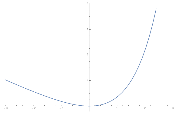

Figure 2 (click to enlarge): Samples from the learned generative model for codes in $[0,1] \times [0,1]$ with step size $0.05$ in both dimensions.
When running the implementation, the output might look as follows:
[Training] created training set
nn.Sequential {
  [input -> (1) -> (2) -> (3) -> (4) -> output]
  (1): nn.Sequential {
    [input -> (1) -> (2) -> (3) -> (4) -> (5) -> (6) -> (7) -> output]
    (1): nn.View(576)
    (2): nn.Linear(576 -> 1152)
    (3): nn.ReLU
    (4): nn.Linear(1152 -> 1152)
    (5): nn.ReLU
    (6): nn.View(1152)
    (7): nn.ConcatTable {
      input
        |`-> (1): nn.Linear(1152 -> 2)
         `-> (2): nn.Linear(1152 -> 2)
         ... -> output
    }
  }
  (2): nn.KullbackLeiblerDivergence
  (3): nn.ReparameterizationSampler
  (4): nn.Sequential {
    [input -> (1) -> (2) -> (3) -> (4) -> (5) -> (6) -> (7) -> output]
    (1): nn.Linear(2 -> 1152)
    (2): nn.ReLU
    (3): nn.Linear(1152 -> 1152)
    (4): nn.ReLU
    (5): nn.Linear(1152 -> 576)
    (6): nn.View(1, 24, 24)
    (7): nn.Sigmoid
  }
}
[Training] 50/31250: 3273.7744824219 | 36.138165675104 | 0.30706121515483 | 0.59900984149426 | -1.4048201445118
[Training] 100/31250: 1825.9491625977 | 107.45124046326 | 0.14986009227112 | 0.99827847599983 | -4.2601121377945
[Training] 150/31250: 1300.8635327148 | 109.24840332031 | 0.15660988058895 | 0.83237507104874 | -4.9025347995758
[Training] 200/31250: 941.38320800781 | 116.9802923584 | 0.1180160830915 | 0.57122075676918 | -4.9226305675507
[Training] 250/31250: 777.5618737793 | 122.0270425415 | 0.28438305184245 | 0.64493700385094 | -5.1193972015381
# ...
The network architecture is printed and every $50$ iterations the following statistics are printed for monitoring:
- Binary cross entropy loss;
- Kullback-Leibler divergence;
- Average mean $\mu(z)$;
- Average standard deviation $\sigma(z)$;
- Average log-variance $l(z)$;
Figure 2 shows an interpolation image. Specifically, the generated images for codes in $[0,1] \times [0,1]$ with step $0.05$ in both dimensions. For short training times, for example $1$ epoch with $3125$ iterations, the reconstructions are not perfect. But it is still visible that the network effectively learns the variation within the dataset, in particular, the translation in height and width.
Outlook
Besides the original variational auto-encoder [], we also discussed denoising variational auto-encoders [] as well as categorical variational auto-encoders [][]. Therefore, the following articles will deal with the extension of the above code template for implementing denoising and vcategorical variational auto-encoders.
- [] D. P. Kingma and M. Welling. Auto-encoding variational bayes. CoRR, abs/1312.6114, 2013.
- [] D. J. Im, S. Ahn, R. Memisevic, and Y. Bengio. Denoising criterion for variational auto-encoding framework. In AAAI Conference on Artificial Intelligence, pages 2059-2065, 2017.
- [] E. Jang, S. Gu, and B. Poole. Categorical reparameterization with gumbel-softmax. CoRR, abs/1611.01144, 2016.
- [] C. J. Maddison, A. Mnih, and Y. W. Teh. The concrete distribution: A continuous relaxation of discrete random variables. CoRR, abs/1611.00712, 2016.