Vanilla variational auto-encoders as introduced in [] consider a Gaussian latent space. As such, all variables are considered independent and continuous. An interesting extension considers discrete latent variables; the, the corresponding prior distribution over the latent space is characterized by independent categorical distributions. In the case of binary latent variables, this reduces to Bernoulli distributions.

In this article, I want to discuss the mathematical background of categorical variational auto-encoders. In addition, this is the third article in my series on variational auto-encoders; check out the first two articles:

• The Mathematics of Variational Auto-Encoders
• Denoising Variational Auto-Encoders

Prerequisites. This article requires basic understanding of linear algebra, probability theory — including conditional probability, Gaussian distributions, Bernoulli distributions and expectations &mdash as well as (convolutional) neural networks. The first two articles on regular variational auto-encoders and denoising variational auto-encoders will also benefit understanding.

Overview

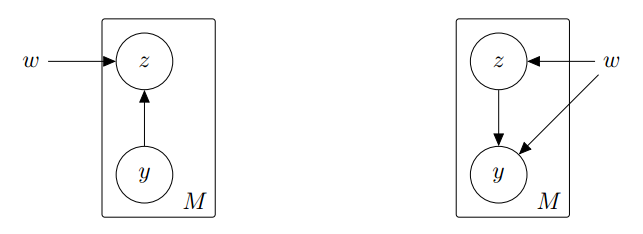
The original variational auto-encoder is based on the more general continuous latent variable model as illustrated in Figure 1. As such, the model is intended to learn a latent space $\mathcal{Z} = \mathbb{R}^Q$ using a given set of samples $\{y_m\} \subseteq \mathcal{Y} = \mathbb{R}^R$ where $Q \ll R$, i.e. a dimensionality reduction. The model consists of the generative model $p(y | z)$ given a fixed prior $p(z)$, and the recognition (inference) model $q(z | y)$. The vanilla variational auto-encoder imposes a unit Gaussian prior

$p(z) = \mathcal{N}(z; 0, I_Q)$

such that the recognition model $q(z | y)$ also needs to be modeled as Gaussian distribution.

Unfortunately, the original variational auto-encoder cannot easily be extended to handle discrete latent variables. Considering the corresponding loss,

$\mathcal{L}_{\text{VAE}} (w) = \text{KL}(q(z|y_m) | p(z)) - \frac{1}{L}\sum_{l = 1}^L \ln p(y_m | z_{l,m})$

where $y_m$ is a training sample and $z_{l,m} = g(\epsilon_{l,m}, y)$ with $\epsilon_{l,m} \sim \mathcal{N}(\epsilon ; 0, I_Q)$. Here, $g$ represents the so-called reparamterization trick:

$z_i = g_i(y, \epsilon_i) = \mu_i(y) + \epsilon_i \sigma_i^2(y)$

which ensures the differentiability of the model with respect to its input. When assuming the latent variables $z$ to be discrete, we would need another reparameterization trick that

• allows sampling from discrete distributions;
• while ensuring differentiability with respect to the model's input.

In the following, we will discuss the special case of Bernoulli (i.e. binary) latent variables based on two recent publications: [] and []. Both papers propose essentially the same reparameterization trick for Bernoulli latent variables.

Bernoulli Variational Auto-Encoder

Assuming Bernoulli latent variables, as in [][], the prior $p(z)$ and the recognition model $q(z|y)$ are modeled as

$p(z) = \prod_{i = 1}^Q \text{Ber}(z_i; 0.5)$

$p(z | y) = \prod_{i = 1}^Q \text{Ber}(z_i; \theta_i(y))$

where $\theta_i(y)$ are predicted using the encoder, given the input $y$. As before, the likelihood is to be optimized during training. As this may be infeasible, the evidence lower bound is optimized isntead. This means for a training sample $y_m$:

$\mathcal{L}_{\text{VAE}} (w) = \text{KL}(q(z|y_m) | p(z)) - \frac{1}{L}\sum_{l = 1}^L \ln p(y_m | z_{l,m})$

where $z_{l,m} \sim q(z|y)$. Again, the Kullback-Leibler divergence can be computed analytically, however, differentiation through the sampling process $z_{l,m} \sim q(z | y)$ is problematic — unfortunately, the reparameterization trick used in the Gaussian case is not applicable anymore.

At this point, Maddison et al. [] and, concurrently, Jang et al. [] propose an alternative reparameterization trick for the more general discrete distribution:

For the discrete reparameterization trick, they additionally considered the so-called Gumbel distribution. For those not familiar with the Gumbel distribution, it is formally defined as follows:

A key insight is that it is very easy to sample from a Gumbel distribution: let $u_k \sim U(0,1)$, then $\epsilon_k = \mu - \beta \log(-\log(u_k))$ is distributed according to $\text{Gu}(\mu, \beta)$. The standard Gumbel distribution also helps to sample from a discrete distribution. Let $\epsilon_{1},\ldots,\epsilon_{K} \sim \text{Gu}(\epsilon; 0, 1)$, then set $z_k = 1$ for

$k = \arg\max_{k} \ln \pi_k + \epsilon_{k}$(1)

and $z$ will be distributed according to a discrete distribution, i.e. $z \sim \text{Dis}(z;\pi)$; this is called the Gumbel trick. Replacing the $\arg\max$ with its smooth counterpart, i.e. the softmax, yields the final reparameterization trick:

$z_k = \frac{\exp(\ln \pi_k + \epsilon_k)}{\sum_{k' = 1}^d \exp(\ln \pi_{k'} + \epsilon_{k'})}$.(2)

Both in [] and in [], an additional temperature parameter, i.e. $\frac{\ln \pi_k + \epsilon_k}{\lambda}$, is added. Then it can be shown that for $\lambda \rightarrow 0$, Equation (2) tends to the real discrete distribution. For simplicity, we neglect the temperature $\lambda$ in the following discussion; in practice, however, the temperature parameter can be useful.

The Bernoulli distribution is merely a special case of the discrete distribution. Specifically, letting $z \sim \text{Ber}(z;\theta)$, $z = 1$ means that

$\ln \theta + \epsilon_1 > \ln (1 - \theta) + \epsilon_2$

where we used Equation (1) with $\pi_1 = \theta$ being the probability of $z = 1$ and $\pi_2 = (1 - \theta)$ the probability of $z = 0$ and made the $\arg\max$ explicit through the inequality. Maddison et al. [] argue that the difference of two Gumbel random variables $\epsilon_1 - \epsilon_2$ is distributed according to a Logistic distribution where we can sample from using

$\epsilon_1 - \epsilon_2 = \ln u - \ln (1 - u)$

with $u \sim U(0,1)$. This can also be verified in []. Thus,

$z = \begin{cases}1&\quad\ln u - \ln (1 - u) + \ln \theta - \ln (1 - \theta) > 0\\0&\quad\text{else}\end{cases}$

which can be made differentiable using a soft thresholding operation such as the sigmoid function. With a change in notation, letting $\epsilon \sim U(0,1)$ this results in

$z_i = g(y, \epsilon) = \sigma\left(\ln \epsilon - \ln (1 - \epsilon) + \ln \theta_i(y) - \ln (1 - \theta_i(y))\right)$(3)

which is the final reparameterization trick used. The remaining framework stays unchanged; the Kullback-Leibler divergence is again computed analytically and the reconstruction error $- \ln p(y | z)$ depends on the exact form of $p(y |z)$ as discussed before.

Practical Considerations

The main difference between a Gaussian variational auto-encoder and the Bernoulli counterpart is the reparameterization trick and the corresponding Kullback-Leibler divergence. The latter can, again, be separated over $1 \leq i \leq Q$ and then be calculated analytically:

$\text{KL}(q(z_i | y) | p(z_i)) = \text{KL}(\text{Ber}(z_i; \theta_i(y)) | \text{Ber}(z_i; 0.5))$

$=\sum_{k \in \{0,1\}} \ln \theta_i(y)^k (1 - \theta_i(y))^{1 - k} - \ln 0.5^k 0.5^{1-k}$(5)

where we use $\text{Ber}(z_i;0.5)$ as prior, i.e. our standard Bernoulli distribution. The gradient with respect to the parameters $\theta_i(y)$ is, as before, added during error backpropagation.

Note that when implemented — in contrast to the vanilla variational auto-encoder — the reparameterization operation needs to be followed by a sigmoid activation before computing the Kullback-Leibler divergence.

Outlook

After discussing the mathematical background of variational auto-encoders, including their denoising variant as well as the case of discrete latent variables, the practical part of this series is going to start with the next article. We will implement all the introduced concepts in Torch.

• [] E. Jang, S. Gu, and B. Poole. Categorical reparameterization with gumbel-softmax. CoRR, abs/1611.01144, 2016.
• [] C. J. Maddison, A. Mnih, and Y. W. Teh. The concrete distribution: A continuous relaxation of discrete random variables. CoRR, abs/1611.00712, 2016.
• [] M. E. Ben-Akiva and S. R. Lerman. Discrete Choice Analysis: Theory and Application to Travel Demand. MIT Press, 1985.