Introduction
$L_p$ constrained adversarial examples as, for example, computed by the original PGD attack [] are sometimes argued to represent an unrealistic threat models. Many attackers might not be able to willing to manipulate individual pixels by tiny amounts of noise. Instead, researchers proposed various alternative types of adversarial examples. Good examples are adversarial patches [][] or adversarial frames []. These are essentially visible patches or frames in/around images that can be manipulated arbitrarily while the remaining image remains unchanged. [] shows how these patches can be printed and fool real computer vision applications. In this article I will present a simple PGD-based attack for computing adversarial patches and frames.
This article is part of a series:
- Monitoring PyTorch Training using Tensorboard
- Loading and Saving PyTorch Models Without Knowing the Architecture in Advance
- 2.56% Test Error on CIFAR-10using PyTorch and AutoAugment
- Lp Adversarial Examples using Projected Gradient Descent in PyTorch
- 47.9% Robust Test Error on CIFAR10 with Adversarial Training and PyTorch
- Generalizing Adversarial Robustness with Confidence-Calibrated Adversarial Training in PyTorch
- Proper Robustness Evaluation of Confidence-Calibrated Adversarial Training in PyTorch
- Distal Adversarial Examples Against Neural Networks in PyTorch
The code for this article can be found on GitHub:
Code on GitHubAdversarial Patches and Frames
As described in this previous article, standard adversarial examples intend to compute an additive perturbation $\delta$ for a given image $x$ that maximizes the cross-entropy loss $\mathcal{L}(f(x + \delta), y)$ of the model $f$ with respect to the true label $y$. More formally,
$\max_{\|\delta\|_p \leq \epsilon} \mathcal{L}(f(x + \delta), y)$
where the perturbation $\delta$ is often constrained in its $L_p$ norm to make sure the perturbation is not visible. Adversarial patches follow a similar idea but allow the perturbation to be visible. Specifically, the perturbation is commonly constrained to a small patch of pixels in the corners of the image. Formally, most works consider a fixed mask $m \in \{0, 1\}^{H\times W\times C}$ with $H, W, C$ being the image height, width and channels. Then, the above optimization problem can be rewritten as:
$\max_{(1-m)\odot x + m \odot \delta \in [0,1]^{H\times W\times C}} \mathcal{L}(f((1-m)\odot x + m \odot \delta), y)$
where $\odot$ denotes element-wise multiplication. With a fixed mask $m$, the same algorithms as used for general adversarial attacks can be used, without the projection of $\delta$ onto the $L_p$-ball — while still making sure that the overall image $(1-m)\odot x + m \odot \delta$ is in $[0,1]$. However, the mask position can also be optimized along the perturbation $\delta$ as done in []. In this article, however, we will just consider random patch locations of fixed (square) size. Alternatively, it is also common to simply allow the adversary to manipulate a frame of fixed size around the image [].
PyTorch Implementation
The adversarial patch implementation in Listing 1 below implements the interface introduced in the previous articles. Essentially, run applies the attack on a set of images given a neural network model and an objective. The objective encodes the loss to be optimized which potentially requires knowledge of the images' labels:
Listing 1: Adversarial patch attack implementation based on a mask generator (see Listing 2).
def run(self, model, images, objective, writer=None, prefix=''):
    """Run adversarial patches attack."""
    super(BatchPatches, self).run(model, images, objective, writer, prefix)
    batch_size, channels, _, _ = images.shape
    is_cuda = common.torch.is_cuda(model)

    # 1. Set up the mask using the mask generator from Listing 2.
    mask_coords = self.mask_gen.random_location(batch_size)
    masks = common.torch.as_variable(self.mask_gen.get_masks(mask_coords, channels).astype(numpy.float32), cuda=is_cuda)
    patches = common.torch.as_variable(numpy.random.uniform(low=0.0, high=1.0, size=images.shape).astype(numpy.float32), cuda=is_cuda, requires_grad=True)

    current_iteration = 0
    success_errors = numpy.ones((batch_size), dtype=numpy.float32) * 1e12
    success_perturbations = numpy.zeros(images.shape, dtype=numpy.float32)

    while current_iteration < self.max_iterations:
        current_iteration += 1

        # 2. Apply the mask and forward pass.
        imgs_patched = (1 - masks)*images + masks*patches
        preds = model(imgs_patched)
        pred_classes = torch.argmax(preds, dim=1)

        # 3. Compute optimization objective and perform backward pass.
        # See previous articles, objective can be the cross-entropy loss and knows the true or target labels.
        error = objective(preds)
        success = objective.success(preds)
        loss = torch.sum(error)
        loss.backward()

        # 4. Keep track of best loss and patches to return after optimization.
        for b in range(batch_size):
            if error[b].item() < success_errors[b]:
                success_errors[b] = error[b].item()
                success_perturbations[b] = (masks[b]*patches[b]).detach().cpu().numpy()

        # Get gradient and update perturbation; make sure overall image is within [0, 1]
        loss_grad = patches.grad
        patches.data = patches - self.base_lr*masks*torch.sign(loss_grad)
        patches.data.clamp_(self.min, self.max)
        patches.grad.data.zero_()

    return success_perturbations, success_errors
- We start by using a mask generator to select random patch masks — this makes it easy to replace patches by frames or change patch locations.
- In search iteration, we first apply the patch as described above: $(1 - m)\odot x + m\odot \delta$.
- Then, the objective is computed — this could be just to maximize cross-entropy loss with respect to the true labels or to create a targeted adversarial patch with specific target labels.
- We keep track of the best adversarial patch to return across all iterations.
The attack is pretty much a standard first-order optimization attack with the additional detail of applying the mask patches. The mask itself is generated using a mask generator such as the below for square patches. This allows to easily use other patches, ranomize locations or use frames instead:
Listing 2: Mask generator for square patches.
class PatchGenerator:
    """Generates a random mask location for applying an adversarial patch to an image."""
    def __init__(self, img_dims, mask_dims, exclude_list=None):
        """Construct patch generator."""
        # 1. Define the set of allowed pixels for the mask location.
        # This could also be limited by, e.g., the central part of the image.
        self.mask_dims = mask_dims
        self.allowed_pixels = set()
        y = 0
        x = 0
        h = img_dims[0] - 1
        w = img_dims[1] - 1
        assert x >= 0 and y >= 0 and h > 0 and w > 0
        assert y + h < self.img_dims[0] and x + w < self.img_dims[1]
        y_range = np.arange(y, y + h - self.mask_dims[0] + 1)
        x_range = np.arange(x, x + w - self.mask_dims[1] + 1)
        pixels = [(y, x) for y in y_range for x in x_range]
        self.allowed_pixels.update(pixels)

    def random_location(self, n=1):
        """Generates n mask coordinates randomly from allowed locations."""
        # 2. Generate some random patch locations from the set of allowed pixels.
        start_pixels = choices(tuple(self.allowed_pixels), k=n)
        return np.array([(y, x, self.mask_dims[0], self.mask_dims[1]) for (y, x) in start_pixels])

    def get_masks(self, mask_coords, n_channels):
        """Gets mask in image shape given mask coordinates."""
        # 3. Convert locations to actual masks.
        assert n_channels >= 1
        batch_size = len(mask_coords)
        masks = np.zeros((batch_size, n_channels, self.img_dims[0], self.img_dims[1]))
        for b in range(batch_size):
            masks[b, :, mask_coords[b][0]:mask_coords[b][0]+self.mask_dims[0],
                  mask_coords[b][1]:mask_coords[b][1]+self.mask_dims[1]] = 1
        return masks
- The simplest patch generator allows to generate patches across the whole image; but we set patches at the top left corner, so all image pixels for which the patch would be partly outside the image are discarded.
- For a batch of size
n, we generate patch locations randomly across all allowed pixels. - The sampled locations are converted to masks using a fixed mask size.
Results
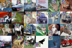
Figure 1: Examples of successful adversarial examples with random patch locations of fixed size on CIFAR10.
| Patches | Frames | ||
| Size | RTE | Size | RTE |
| 4 | 0.064 | 1 | 0.316 |
| 6 | 0.1514 | 2 | 0.7642 |
| 8 | 0.297 | 3 | 0.9226 |
| 10 | 0.4306 | ||
| 12 | 0.5854 | ||
Table 1: Robust test error for adversarial patches and adversarial frames of varying sizes against a normal, non-robust model.
I ran experiments on CIFAR10 using a normally trained, non-robust WRN-28-10. As attacks, I considered adversarial (square) patches of varying size as well as adversarial frames of varying thickness. These were computed on the first $1000$ test examples and robust test error (RTE) denotes the fraction of examples where the model mis-classifies the adversial images, see Table 1. Even normally trained models are quite robust against small adversarial patches or 1-pixel adversarial frames. However, this is also due to the small image size, where even patches of size $8 \times 8$ look quite distracting. Some examples are shown in Figure 1.
Conclusion
Overall, adversarial patches with fixed patch locations are fairly easy to implement following a basic projected gradient descent scheme. The above implementation has the advantage that it operates purely on a mask, making the implementation agnostic to how the mask is generated, whether it is a patch, a few individual pixels or a frame. Typically, normally trained models are more robust against small patches that standard adversarial examples, but this is partly due to the small image size on CIFAR10. In the next article, I will show a final version of adversarial examples, so-called adversarial transformations.
- [] Aleksander Madry, Aleksandar Makelov, Ludwig Schmidt, Dimitris Tsipras, Adrian Vladu. Towards Deep Learning Models Resistant to Adversarial Attacks. ICLR (Poster) 2018.
- [] Tom B. Brown, Dandelion Mané, Aurko Roy, Martín Abadi, Justin Gilmer: Adversarial Patch. CoRR abs/1712.09665 (2017).
- [] Sukrut Rao, David Stutz, Bernt Schiele: Adversarial Training Against Location-Optimized Adversarial Patches. ECCV Workshops (5) 2020: 429-448.
- [] Michal Zajac, Konrad Zolna, Negar Rostamzadeh, Pedro O. Pinheiro: Adversarial Framing for Image and Video Classification. AAAI 2019: 10077-10078.