Introduction
Since their discovery [], research on adversarial examples has exploded. Various different attacks have been proposed, but projected gradient descent (PGD) based attacks [][][] have become pretty standard in terms of robustness evaluation. Originally, the PGD attack was focussed on $L_\infty$-constrained adversarial examples. However, the concept can also be used to generate arbitrary $L_p$ adversarial examples such that improvements/changes of the PGD algorithm, in general, are widely applicable.
In this article, I want to present my PyTorch implementation of projected gradient descent. The implementation allows batch computation of arbitrary $L_p$ adversarial examples for evaluation or adversarial training []. Furthermore, the implementation comes with monitoring, in console or via TensorBoard, for debugging. Finally, the implementation also includes three crucial improvements: First, instead of early sopping or returning the final adversarial example (after $T$ iterations), the algorithm returns the worst-case adversarial examples across all iterations. Second, momentum is used for the gradient updates, following []. Third, backtracking can be used to ensure that gradient updates do not "weaken" the adversarial example by automatically reducing learning rate throughout iterations.
This article is part of a series of articles:
- Monitoring PyTorch Training using Tensorboard
- Loading and Saving PyTorch Models Without Knowing the Architecture in Advance
- 2.56% Test Error on CIFAR-10using PyTorch and AutoAugment
Among others, the previous articles show how to obtain near state-of-the-art performance on CIFAR-10 []. In a future article, I will show how to combine this with the PGD attack presented in this article to perform adversarial training [].
The code for this article can be found on GitHub:
Code on GitHubProjected Gradient Descent
I will go through the basic steps of the projected gradient descent (PGD) algorithm using the example of $L_\infty$ adversarial examples. PGD is a first-order optimization technique in order to minimize some objective $\mathcal{F}$. However, in the context of adversarial examples, it is usually used to maximize $\mathcal{F}$. Thus, projected gradient ascent is often the more appropriate description (nevertheless, I will follow common practice and refer to the algorithm as PGD). This is because the objective $\mathcal{F}$ is typically chosen to be the cross-entropy loss $\mathcal{L}$:
$\mathcal{F}(x + \delta, y) = \mathcal{L}(f(x + \delta), y)$
where $\delta$ represents the additive (adversarial) perturbation to be added to .
PGD maximizes the objective $\mathcal{F}$ by taking steps along the gradient's direction. Remember: the gradient $\nabla \mathcal{F}$ points into the direction of the fastest increase in $\mathcal{F}$. As we aim to optimize over the perturbation $\delta$, each iteration $t$ of PGD performs the following update with learning rate $\gamma$:
$\delta^{(t)} = \delta^{(t - 1)} + \gamma \nabla \mathcal{F}(x + \delta^{(t - 1)}, y)$.(2)
In practice, the gradient is not used as is though. Often, the gradient is normalized which makes it "easier to work with". When the model performs well, the cross-entropy loss $\mathcal{L}(f(x), y)$ is typically close to zero. This is also the case for many examples near $x$. Thus, the gradient may also be close to zero such that the updates in Equation (2) are "meaningless". When talking about normalizing the gradient, researchers usually refer to the steepest descent direction (or ascent in our case). For $L_\infty$ this means using the signed gradient:
$\delta^{(t)} = \delta^{(t - 1)} + \gamma \text{sign}\left(\nabla \mathcal{F}(x + \delta^{(t - 1)}, y)\right)$
The derivation is more involved, but details can be found (among other resources) here.
After each update, the current perturbation $\delta^{(t)}$ is projeted onto the set of constraints. For adversarial examples computed on images, this is typically a constraint like $x_i + \delta^{(t)}_i \in [0,1]$ assuming that all images are normalized to $[0,1]$ ($i$ indexes individual pixels). Additionally, adversarial examples are constrained to an $L_\infty$-ball of size $\epsilon$ around $x$. These constraints translate to the following operations:
$\delta^{(t)} := \max(-\epsilon, \min(\epsilon, \delta^{(t)}))$(4)
$\delta^{(t)} := \min(1 - x, \delta^{(t)})$(5)
$\delta^{(t)} := \max(0 - x, \delta^{(t)})$(6)
where we assume element-wise application of $\max$ and $\min$ as well as the subtraction. The projection onto the $\epsilon$-ball depends on the norm used (here, $L_\infty$).
Momentum: [] additionally use momentum for PGD: instead of "just" taking the gradient $\nabla \mathcal{F}(x + \delta^{(t)}, y)$ in each iteration, the gradient is augmented by the direction of previous iterations. Using $g^{(t)}$ to denote the gradient $\nabla \mathcal{F}(x + \delta^{(t)}, y)$, the new update is computed as:
$g^{(t)} = \beta g^{(t - 1)} + (1 - \beta)g^{(t)}$
where $g^{(-)}$ is initialized as $0$ (i.e., no momentum is used in the first iteration $t = 0$). It is common to use heavy momentum, for example, with $\beta = 0.9$. Generally, momentum will speed up optimization and achieve "better" adversarial examples by avoiding oscillation and other optimization difficulties.
Backtracking: In [], I additionally used a backtracking scheme that helps to automatically select the learning rate. Such approaches have also become popular in more recent attacks []. Essentially, this means that the update $g^{(t)}$ is "tested" before applying it. Specifically, if the update does not improve objective, it is not applied and the learning rate is reduced instead. For this, an additional hyper-parameter $\alpha$ is introduced such that $\gamma = \gamma/\alpha$ if the update does not improve the objective. As backtracking requires an additional forward pass in each iteration, it really depends on the defense to be attacked to decide whether backtracking is necessary.
Best vs. Last Iteration: Instead of running PGD and using $\delta^{(T - 1)}$, corresponding to the final iteration $T$, as adversarial noise, [] as well as later attacks [] also allow to use the $\delta^{(t)}$ corresponding to the best iteration $t$. This is achieved by taking track of the best adversarial noise during training.
Algorithm 1: Projected gradient descent (PGD) for generating $L_\infty$ adversarial examples. The algorithm assumes a single input/label pair $x, y$, but can easily be implemented as batch algorithm.
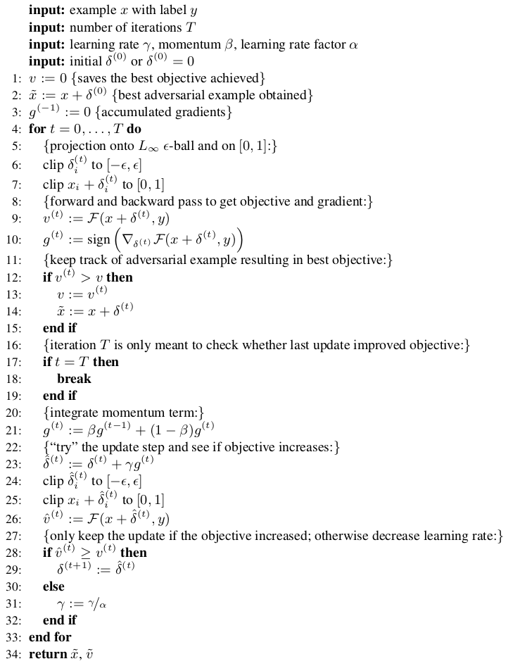
For $L_\infty$ adversarial examples, the whole algorithm is summarized above in Algorithm 1. This algorithm is formulated for an individual example, however, it can easily be implemented using batch operations. In this case, however, it is important to use individual learning rates per example. Moreover, the algorithm applies the projections first, then the update step and then applies backtracking. This is useful when starting with an initialization $\delta^{(0)} \neq 0$ that does not fulfill the constraints.
$L_p$ Initializations, Projections and Normalization
The PGD variant described above obtains adversarial examples with $\delta$ constrained to $\|\delta\|_\infty \leq \epsilon$. However, the same algorithm can also be used for $L_2$, $L_1$ and $L_0$ adversarial examples just. To this end, the following components need to be adapted:
- Initialization of $\delta^{(0)}$
- Gradient normalization of $g^{(t)}$
- Projection onto $\|\delta\|_p \leq \epsilon$
Of course, the constraint $\epsilon$ also has to be adapted, see for example this article on meaningful choices. In the following, I want to cover all three aspects for $L_2$, $L_1$ and $L_0$ adversarial examples:
Initialization for $L_\infty$, $L_2$ and $L_1$ follows a simple equation:
$\delta = u \epsilon \frac{\delta'}{\|\delta'\|_2}$
with $u \sim U(0,1)$ sampled from a uniform distribution in $[0,1]$ and $\delta' \sim \mathcal{N}(0,1)$ sampled from a standard Gaussian distribution. Essentially, this initialization first sampled a direction (using the Gaussian sample), then normalizes it and then uniformly chooses the length/magnitude. Only for $L_0$, initialization needs to be adapted a bit. I found sampling $\frac{2}{3}\epsilon /(HWC)$ pixels and setting them to uniform values $u \sim U(0,1)$ to work well in practice.
Gradient Normalization for $L_\infty$ boils down to taking the sign of the gradient. For $L_2$, $L_1$ and $L_0$, I divide by the $L_2$ norm, only keep the $1\%$-largest values and divide by the $L_1$ norm, respectively.
The projection results in clipping all pixels to $[-\epsilon,\epsilon$ for the $L_\infty$ norm. For the $L_2$ norm, $\delta$ is normalized by its $L_2$ norm if $\|\delta\|_2 > \epsilon$. For $L_1$, the projection is more involved, but luckily there are implementations available. Finally, for $L_0$, only the $\epsilon$-largest values are kept (note that this involves sorting).
Note that only these three aspects need to be replaced in order to compute, e.g., $L_2$ adversarial examples instead of $L_\infty$ ones. Thus, the implementation shown in the following will be very modular.
PyTorch Implementation
I will start by describing the general interface of an adversarial attack. Specifically, Listing 1 shows an attack interface that I will work with. This allows to also implement other attacks without changing the underlying code that runs the attack:
Listing 1: Attack interface to be used by the PGD implementation discussed later.
class Attack:
    # 1. The constructor will be used to set some hyper-parameters.
    def __init__(self):
        self.progress = None
        """ (common.progress.ProgressBar) Progress bar. """

    # 2. This will actually run the attack, given a model and a set of images.
    # Note that the objective to be optimized is also provided as argument.
    # The true labels, if required for the attack, are provided through the objective.
    def run(self, model, images, objective, writer=common.summary.SummaryWriter(), prefix=''):
        assert model.training is False
        assert isinstance(images, torch.autograd.Variable)
        assert isinstance(objective, Objective)
        assert common.torch.is_cuda(model) == common.torch.is_cuda(images)
        writer.add_text('%sobjective' % prefix, objective.__class__.__name__)
- The constructor will later be used to initialize the hyper-parameters of the attack. Note that the constructor does not take into account the model or images tobe attacked.
runwill actually compute adversarial examples for a given models, set of images and objective. The objective also contains the true labels if required.
Before considering the actual PGD implementation, I will describe the objective to be optimized. Remember that standard PGD maximizes cross-entropy loss. My PGD implementation, however, expects an objective to be minimized:
Listing 2: The objective defines what we want to optimize as part of the PGD attack.
class Objective:
    def __init__(self):
        self.true_classes = None
        """ (torch.autograd.Variable) True classes. """
        self.target_classes = None
        """ (torch.autograd.Variable) Target classes. """

    # 1. The true or target classes (for targeted attacks) are set here and not provided to the attack's run method.
    def set(self, true_classes=None, target_classes=None):
        if target_classes is not None:
            assert true_classes is not None
        if true_classes is not None and target_classes is not None:
            assert target_classes.size()[0] == self.true_classes.size()[0]

        self.true_classes = true_classes
        self.target_classes = target_classes

    def __call__(self, logits, perturbations=None):
        raise NotImplementedError()

    # 2. The objective is also used to provide some metrics to be monitored during the attack:
    def success(self, logits):
        if self.true_classes is not None:
            return torch.clamp(torch.abs(torch.max(common.torch.softmax(logits, dim=1), dim=1)[1] - self.true_classes), max=1)
        else:
            return torch.max(common.torch.softmax(logits, dim=1), dim=1)[0]


# 3. This objective just maximizes the cross-entropy loss.
class UntargetedF0Objective(Objective):
    def __init__(self, loss=common.torch.classification_loss):
        self.loss = loss
        """ (callable) Loss. """

    def __call__(self, logits, perturbations=None):
        assert self.loss is not None
        return -self.loss(logits, self.true_classes, reduction='none')
- The objective not only defines what to be optimized, but also holds the true or target classes if required. Note that not all attacks might need knowledge about the true class, for example, to avoid label leaking or for distal adversarial examples.
- It is also used to provide meaningful metrics that are monitored throughout the optimization such as the success rate of the attack.
- Maximizing cross-entropy loss translates to minimizing the negative cross-entropy loss. Note that only the
__call__methods needs to be overridden for this.
Note that this way of defining the objective to be optimized allows a wide variety of objectives and supports both untargeted and targeted attacks.
Now, Listing 3 provides the core of the PGD algorithm by implementing the run method of our Attack attack interface, closely following Algorithm 1 but implemented on mini-batches of examples.
Listing 3: The actual PGD implementation.
def run(self, model, images, objective, writer=common.summary.SummaryWriter(), prefix=''):
    # some asserts ...
    is_cuda = common.torch.is_cuda(model)

    # 1. Initialize the adversarial perturbations as well as learning rates for each example.
    self.perturbations = torch.from_numpy(numpy.zeros(images.size(), dtype=numpy.float32))
    if self.initialization is not None:
        self.initialization(images, self.perturbations)
    if is_cuda:
        self.perturbations = self.perturbations.cuda()

    batch_size = self.perturbations.size()[0]
    success_errors = numpy.ones((batch_size), dtype=numpy.float32)*1e12
    success_perturbations = numpy.zeros(self.perturbations.size(), dtype=numpy.float32)

    self.lrs = torch.from_numpy(numpy.ones(batch_size, dtype=numpy.float32) * self.base_lr)
    if is_cuda:
        self.lrs = self.lrs.cuda()

    self.perturbations = torch.autograd.Variable(self.perturbations, requires_grad=True)
    self.gradients = torch.zeros_like(self.perturbations)

    for i in range(self.max_iterations + 1):
        # Zero the gradient, as they are acculumated in PyTorch!
        if i > 0:
            self.perturbations.grad.data.zero_()

        # 2. Apply projections if necessary.
        if self.projection is not None:
            self.projection(images, self.perturbations)

        # 3. Forward pass to obtain the logits and compute the error using the objective.
        # Note that this implementation also allows to penalize the L_p norm in addition to the objective.
        output_logits = model(images + self.perturbations)
        error = self.c*self.norm(self.perturbations) + objective(output_logits, self.perturbations)

        # 4. Check if the perturbations improved the objective
        norm = self.norm(self.perturbations)
        for b in range(batch_size):
            if error[b].item() < success_errors[b]:
                success_errors[b] = error[b].cpu().item()
                success_perturbations[b] = self.perturbations[b].detach().cpu().numpy()

        # Quick hack for handling the last iteration correctly.
        if i == self.max_iterations:
            break

        # 5. Backward pass and gradient computation including momentum:
        torch.sum(error).backward()
        gradients = self.perturbations.grad.clone()

        if self.normalized:
            self.norm.normalize(gradients)
        self.gradients.data = self.momentum*self.gradients.data + (1 - self.momentum)*gradients.data

        # 6. Perform backtracking if requested:
        if self.backtrack:
            next_perturbations = self.perturbations - torch.mul(common.torch.expand_as(self.lrs, self.gradients), self.gradients)
            #assert not torch.any(torch.isnan(self.lrs))
            #assert not torch.any(torch.isnan(next_perturbations))

            if self.projection is not None:
                self.projection(images, next_perturbations)

            next_output_logits = model(images + next_perturbations)
            next_error = self.c * self.norm(next_perturbations) + objective(next_output_logits, next_perturbations)

            # Update learning rate if requested.
            for b in range(batch_size):
                if next_error[b].item() <= error[b]:
                    self.perturbations[b].data -= self.lrs[b]*self.gradients[b].data
                else:
                    self.lrs[b] = max(self.lrs[b] / self.lr_factor, 1e-20)
        else:
            self.perturbations.data -= torch.mul(common.torch.expand_as(self.lrs, self.gradients), self.gradients)

    return success_perturbations, success_errors
- The perturbations $\delta$ for each image in the batch
imagesare initialized usingself.initialization— this will be implemented depending on the $L_p$ norm we want to compute adversarial examples for. - In the beginning of each iteration, we apply the projects. Again,
self.projectionis implemented depending on which $L_p$ projections need to be applied. Usually, this will also include a box projection such that $\tilde{x} = x + \delta \in [0,1]$. - We forward the adversarial examples,
images + self.perturbations, and compute the error which is done using one of the objectives described in Listing 2. - After the forward pass, we check whether the last update improved the objective. If so, the corresponding perturbation is remembered. Afterwards, if this is supposed to be the last iteration, we break the loop.
- If this was not the last iteration, we compute the gradients using a backward pass. Additionally, the gradient is normalized using
self.norm.normalizeand momentum is applied ifself.momentum > 0. - Backtracking involves an additional forward pass, including the projections beforehand. Then, if the objective is improved, the update is applied. If not, the learning rate is reduced by
self.lr_factor. Note that this is done per example individually.
Modularity: To actually run this PGD implementation, we need the following missing ingredients: initialization, projection and gradient normalization. All of these are implemented using separate class interfaces that ensure a high degree of modularity:
Listing 4: Initialization, gradient normalization and projections.
class Initialization:
    def __call__(self, images, perturbations):
        raise NotImplementedError()


# 1. Example for the L_infty initialization that implements the above interface.
class LInfUniformNormInitialization(Initialization):
    def __init__(self, epsilon):
        self.epsilon = epsilon

    def __call__(self, images, perturbations):
        perturbations.data = torch.from_numpy(common.numpy.uniform_norm(perturbations.size()[0], numpy.prod(perturbations.size()[1:]), epsilon=self.epsilon, ord=float('inf')).reshape(perturbations.size()).astype(numpy.float32))


class Norm:
    def __call__(self, perturbations):
        raise NotImplementedError()

    def normalize(self, gradients):
        raise NotImplementedError()


# 2. Example of the L_infty norm that also implement gradient normalization.
class LInfNorm(Norm):
    def __call__(self, perturbations):
        return torch.max(torch.abs(perturbations.view(perturbations.size()[0], -1)), dim=1)[0]

    def normalize(self, gradients):
        gradients.data = torch.sign(gradients.data)


class Projection:
    def __call__(self, images, perturbations):
        raise NotImplementedError()


# 3. This allows to apply multiple projections in sequence.
# Usually this will be a box projection onto [0,1] and a L_p projection.
class SequentialProjections(Projection):
    def __init__(self, projections):
        assert isinstance(projections, list)
        assert len(projections) > 0
        for projection in projections:
            assert isinstance(projection, Projection)

        self.projections = projections

    def __call__(self, images, perturbations):
        for projection in self.projections:
            projection(images, perturbations)


# 4. The box projection that can be used to ensure that adversarial examples are in [0,1].
class BoxProjection(Projection):
    def __init__(self, min_bound=0, max_bound=1):
        assert isinstance(min_bound, float) or isinstance(min_bound, int) or min_bound is None
        assert isinstance(max_bound, float) or isinstance(max_bound, int) or max_bound is None

        self.min_bound = min_bound
        self.max_bound = max_bound

    def __call__(self, images, perturbations):
        if self.max_bound is not None:
            perturbations.data = torch.min(torch.ones_like(perturbations.data) * self.max_bound - images.data, perturbations.data)
        if self.min_bound is not None:
            perturbations.data = torch.max(torch.ones_like(perturbations.data)*self.min_bound - images.data, perturbations.data)


# 5. Example of the L_infty projection.
class LInfProjection(Projection):
    def __init__(self, epsilon):
        self.epsilon = epsilon

    def __call__(self, images, perturbations):
        perturbations.data = common.torch.project_ball(perturbations.data, self.epsilon, ord=float('inf'))
- Initializations for the different $L_p$ norms implement the
Initializationinterface. I provide an example for the $L_\infty$ projection applied using the__call__method. - Gradient normalization is implemented by the
Norminterface. As example, I include the implementation for the $L_\infty$ norm. - Projections implement the
Projectioninterface and theSequentialProjectionclass allows to apply several projections. This is generally the case as we want to enforce both a $L_p$ constraint and a box constraint. - The box constraint projects the adversarial examples to $[0,1]$.
- The $L_\infty$ projection projects the adversarial perturbation onto $\|\delta\|\leq \epsilon$.
Implementations for other $L_p$ norms can be found in the repository.
Monitoring: For debugging and evaluation it can be helpful to integrate some monitoring. In my implementation, this is done by adding Listing 5 after step 5 of Listing 3:
Listing 5: Add monitoring to the PGD implementation.
# 1. Compute gradient magnitudes and metrics provided by the objective.
gradient_magnitudes = torch.mean(torch.abs(gradients.view(batch_size, -1)), dim=1)/self.perturbations.size()[0]
successes = objective.success(output_logits)
true_confidences = objective.true_confidence(output_logits)
target_confidences = objective.target_confidence(output_logits)

# 2. For each example individually, record these key metrics using a summary writer (e.g., TensorBoard writer).
for b in range(batch_size):
    writer.add_scalar('%ssuccess_%d' % (prefix, b), successes[b], global_step=i)
    writer.add_scalar('%strue_confidence_%d' % (prefix, b), true_confidences[b], global_step=i)
    writer.add_scalar('%starget_confidence_%d' % (prefix, b), target_confidences[b], global_step=i)
    writer.add_scalar('%slr_%d' % (prefix, b), self.lrs[b], global_step=i)
    writer.add_scalar('%serror_%d' % (prefix, b), error[b], global_step=i)
    writer.add_scalar('%snorm_%d' % (prefix, b), norm[b], global_step=i)
    writer.add_scalar('%sgradient_%d' % (prefix, b), gradient_magnitudes[b], global_step=i)
# 3. In addition, the progress can be monitored in the command line.
if self.progress is not None:
    self.progress('attack', i, self.max_iterations, info='success=%g error=%.2f norm=%g lr=%g' % (
        torch.sum(successes).item(),
        torch.mean(error).item(),
        torch.mean(norm).item(),
        torch.mean(self.lrs).item(),
    ), width=10)
- For monitoring, gradient magnitude as well as success rate and the confidence of adversarial examples are useful.
- These metrics are recorded for each example individually using a summary writer as shown in this previous article. This can, for example, be a PyTorch TensorBoard writer.
- In addition, progress can be monitored in the command line, see the repository for a possible implementation.
Results
As example, I will apply this PGD implementation for $L_\infty$, $L_2$ and $L_1$ against the WRN-28-10 trained in this previous article. Table 1 shows that the model is not robust at all against these attacks:
| Attack | (Robust) Test Error |
|---|---|
| None | 2.83% |
| $L_\infty$, $\epsilon = 0.03$ | 100.00% |
| $L_2$, $\epsilon = 0.5$ | 98.39% |
| $L_1$, $\epsilon = 10$ | 78.88% |
Table 1: Adversarial robustness against various $L_p$ adversarial attacks.
Note that this only runs PGD once for each example for $T = 7$ iterations. Evaluation was done on the first $1000$ test examples and on adversarial examples, the robust test error is computed as the fraction of examples that are either mis-classified or successfully attacked (i.e., attack switches label). Just increasing the number of iterations to $T = 20$, however, will also increase robust test error for $L_1$ attacks to $94.08\%$.
Conclusion
Overall, PGD is a simple but powerful algorithm to compute adversarial examples with different $L_p$ constraints. Generally, even with few iterations, these attacks can fool deep neural networks almost always. In later articles, I will built on this PGD implementation and show how to train models robust against such adversarial examples.
- [] Christian Szegedy, Wojciech Zaremba, Ilya Sutskever, Joan Bruna, Dumitru Erhan, Ian J. Goodfellow, Rob Fergus. Intriguing properties of neural networks. ICLR (Poster) 2014.
- [] Aleksander Madry, Aleksandar Makelov, Ludwig Schmidt, Dimitris Tsipras, Adrian Vladu. Towards Deep Learning Models Resistant to Adversarial Attacks. ICLR (Poster) 2018.
- [] Yinpeng Dong, Fangzhou Liao, Tianyu Pang, Hang Su, Jun Zhu, Xiaolin Hu, Jianguo Li. Boosting Adversarial Attacks With Momentum. CVPR 2018: 9185-9193.
- [] David Stutz, Matthias Hein, Bernt Schiele. Confidence-Calibrated Adversarial Training: Generalizing to Unseen Attacks. ICML 2020: 9155-9166.
- [] Alex Krizhevsky. Learning Multiple Layers of Features from Tiny Images. 2009.
- [] rancesco Croce, Matthias Hein. Reliable evaluation of adversarial robustness with an ensemble of diverse parameter-free attacks. ICML 2020: 2206-2216.