Introduction
Computer vision benchmarks such as MNIST [] or CIFAR-10 [] are wide-spread within in research across various different task. However, independent of the task being tackled, it is nice — and often expected — to start with state-of-the-art performance as baseline. On MNIST, for example, this is rather easy to achieve and results are quite stable across neural network architectures and learning hyper-parameters. For CIFAR-10, in contrast, obtaining state-of-the-art performance can be time consuming and performance is more dependent on hyper-parameters.
In this article, I want to share a PyTorch setup that achieves 2.56% test error on the CIFAR-10 test set, using a Wide ResNet (WRN-28-10) and only data augmentation using AutoAugment and CutOut. According to Papers with Code, this is still roughly 2% shy of the current state-of-the-art, but the setup is simple and generalizes quite well across architectures.
This article is part of a series of articles. Specifically, the code is based on the training procedure with TensorBoard logging discussed previously:
- Monitoring PyTorch Training using Tensorboard
- Loading and Saving PyTorch Models Without Knowing the Architecture in Advance
The code corresponding to this article can be found on GitHub:
Code on GitHubAutoAugment and CutOut
Data augmentation is among the easiest ways to improve generalization, i.e., performance on the test set. Recently, AutoAugment [] and its variants improved performance on various datasets. Specifically, AutoAugment automatically searches for "improved" data augmentation strategies across a large variety of individual augmentation operations. These operations include transformations such as translation, shear or rotation as well as several color and brightness operations (equalizing, inversion, constrat changes etc.) — the details can be found in the appendix of []. On CIFAR-10, for example, the optimal data augmentation contains 24 of these operations. Similar AutoAugment policies are provided for, e.g., SVHN [] or ImageNet [].
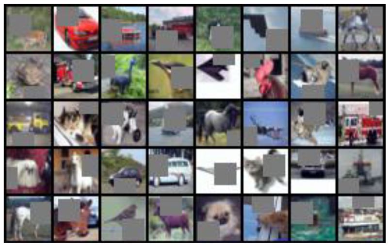
Figure 1: Examples of CutOut on CIFAR-10 from [].
Another easy-to-use data augmentation strategy, going beyond the classical random flipping and rotating, is CutOut []. Here, random patches in the image are cut out and replaced by the mean color image (mean color across all training images, usually gray), as illustrated in Figure 1. The idea is that the network learns to utilizes a variety of features within images depending on which part is cut out — on CIFAR-10, for examples, patches of $16 \times 16$ are usually used.
Luckily, there are PyTorch implementations for both AutoAugment and CutOut avilable on GitHub: DeepVoltaire/AutoAugment and uoguelph-mlrg/Cutout.
AutoAugment
As mentioned, AutoAugment considers a wide range of possible data augmentations. Specifically, $14$ different transformations are defined as so-called sub-policies:
Listing 1: Implementation of sub-policies, i.e., individual data transformations, for AutoAugment.
class SubPolicy(object):
    def __init__(self, p1, operation1, magnitude_idx1, p2, operation2, magnitude_idx2, fillcolor=(128, 128, 128)):
        ranges = {
            "shearX": numpy.linspace(0, 0.3, 10),
            "shearY": numpy.linspace(0, 0.3, 10),
            "translateX": numpy.linspace(0, 150 / 331, 10),
            "translateY": numpy.linspace(0, 150 / 331, 10),
            "rotate": numpy.linspace(0, 30, 10),
            "color": numpy.linspace(0.0, 0.9, 10),
            "posterize": numpy.round(numpy.linspace(8, 4, 10), 0).astype(numpy.int),
            "solarize": numpy.linspace(256, 0, 10),
            "contrast": numpy.linspace(0.0, 0.9, 10),
            "sharpness": numpy.linspace(0.0, 0.9, 10),
            "brightness": numpy.linspace(0.0, 0.9, 10),
            "autocontrast": [0] * 10,
            "equalize": [0] * 10,
            "invert": [0] * 10
        }

        # from https://stackoverflow.com/questions/5252170/specify-image-filling-color-when-rotating-in-python-with-pil-and-setting-expand
        def rotate_with_fill(img, magnitude):
            rot = img.convert("RGBA").rotate(magnitude)
            return Image.composite(rot, Image.new("RGBA", rot.size, (128,) * 4), rot).convert(img.mode)

        func = {
            "shearX": lambda img, magnitude: img.transform(
                img.size, Image.AFFINE, (1, magnitude * random.choice([-1, 1]), 0, 0, 1, 0),
                Image.BICUBIC, fillcolor=fillcolor),
            "shearY": lambda img, magnitude: img.transform(
                img.size, Image.AFFINE, (1, 0, 0, magnitude * random.choice([-1, 1]), 1, 0),
                Image.BICUBIC, fillcolor=fillcolor),
            "translateX": lambda img, magnitude: img.transform(
                img.size, Image.AFFINE, (1, 0, magnitude * img.size[0] * random.choice([-1, 1]), 0, 1, 0),
                fillcolor=fillcolor),
            "translateY": lambda img, magnitude: img.transform(
                img.size, Image.AFFINE, (1, 0, 0, 0, 1, magnitude * img.size[1] * random.choice([-1, 1])),
                fillcolor=fillcolor),
            "rotate": lambda img, magnitude: rotate_with_fill(img, magnitude),
            "color": lambda img, magnitude: ImageEnhance.Color(img).enhance(1 + magnitude * random.choice([-1, 1])),
            "posterize": lambda img, magnitude: ImageOps.posterize(img, magnitude),
            "solarize": lambda img, magnitude: ImageOps.solarize(img, magnitude),
            "contrast": lambda img, magnitude: ImageEnhance.Contrast(img).enhance(
                1 + magnitude * random.choice([-1, 1])),
            "sharpness": lambda img, magnitude: ImageEnhance.Sharpness(img).enhance(
                1 + magnitude * random.choice([-1, 1])),
            "brightness": lambda img, magnitude: ImageEnhance.Brightness(img).enhance(
                1 + magnitude * random.choice([-1, 1])),
            "autocontrast": lambda img, magnitude: ImageOps.autocontrast(img),
            "equalize": lambda img, magnitude: ImageOps.equalize(img),
            "invert": lambda img, magnitude: ImageOps.invert(img)
        }

        self.p1 = p1
        self.operation1 = func[operation1]
        self.magnitude1 = ranges[operation1][magnitude_idx1]
        self.p2 = p2
        self.operation2 = func[operation2]
        self.magnitude2 = ranges[operation2][magnitude_idx2]


    def __call__(self, img):
        if random.random() < self.p1: img = self.operation1(img, self.magnitude1)
        if random.random() < self.p2: img = self.operation2(img, self.magnitude2)
        return img
Each sub-policy consists of two transformations, specified through operation1 and operation2 which are applied sequentially with probabilities p1 and p2, respectively (see the __call__ method). The possible operations include shear, translation, rotation, contrast changes and brightness changes, among others; for each transformation a possible range of parameters is defined. For example, the rotation is applied at 10 discrete steps between $0$ and $30$ degrees. The implementation of most transformations is straight-forward and just uses functionality provided by PIL. For some operations, including rotation, translation or shear, the color to be filled in is defined by fillcolor and will, in practice, be set to the mean color on the training set./p>
AutoAugment randomly selects one of multiple sub-policies. These sub-policies have been optimized to yield the best performance. For CIFAR-10, the policy is defined as follows:
Listing 2: The CIFAR-10 AutoAugment policy consists of multiple individual sub-policies; a random sub-policy is selected for each image.
class CIFAR10Policy(object):
    def __init__(self, fillcolor=(128, 128, 128)):
        self.policies = [
            SubPolicy(0.1, "invert", 7, 0.2, "contrast", 6, fillcolor),
            SubPolicy(0.7, "rotate", 2, 0.3, "translateX", 9, fillcolor),
            SubPolicy(0.8, "sharpness", 1, 0.9, "sharpness", 3, fillcolor),
            SubPolicy(0.5, "shearY", 8, 0.7, "translateY", 9, fillcolor),
            SubPolicy(0.5, "autocontrast", 8, 0.9, "equalize", 2, fillcolor),

            SubPolicy(0.2, "shearY", 7, 0.3, "posterize", 7, fillcolor),
            SubPolicy(0.4, "color", 3, 0.6, "brightness", 7, fillcolor),
            SubPolicy(0.3, "sharpness", 9, 0.7, "brightness", 9, fillcolor),
            SubPolicy(0.6, "equalize", 5, 0.5, "equalize", 1, fillcolor),
            SubPolicy(0.6, "contrast", 7, 0.6, "sharpness", 5, fillcolor),

            SubPolicy(0.7, "color", 7, 0.5, "translateX", 8, fillcolor),
            SubPolicy(0.3, "equalize", 7, 0.4, "autocontrast", 8, fillcolor),
            SubPolicy(0.4, "translateY", 3, 0.2, "sharpness", 6, fillcolor),
            SubPolicy(0.9, "brightness", 6, 0.2, "color", 8, fillcolor),
            SubPolicy(0.5, "solarize", 2, 0.0, "invert", 3, fillcolor),

            SubPolicy(0.2, "equalize", 0, 0.6, "autocontrast", 0, fillcolor),
            SubPolicy(0.2, "equalize", 8, 0.6, "equalize", 4, fillcolor),
            SubPolicy(0.9, "color", 9, 0.6, "equalize", 6, fillcolor),
            SubPolicy(0.8, "autocontrast", 4, 0.2, "solarize", 8, fillcolor),
            SubPolicy(0.1, "brightness", 3, 0.7, "color", 0, fillcolor),

            SubPolicy(0.4, "solarize", 5, 0.9, "autocontrast", 3, fillcolor),
            SubPolicy(0.9, "translateY", 9, 0.7, "translateY", 9, fillcolor),
            SubPolicy(0.9, "autocontrast", 2, 0.8, "solarize", 3, fillcolor),
            SubPolicy(0.8, "equalize", 8, 0.1, "invert", 3, fillcolor),
            SubPolicy(0.7, "translateY", 9, 0.9, "autocontrast", 1, fillcolor)
        ]

    def __call__(self, img):
        policy_idx = random.randint(0, len(self.policies) - 1)
        return self.policies[policy_idx](img)
Example images of CIFAR-10 with AutoAugment applied are shown in Figure 1. Note that the augmentations can be rather strong and might include minor artifacts.
CutOut
CutOut is conceptionally easy: for a given size $s$, randomly cutout a $s \times s$ patch of the image and replace it by the mean image color (across the training set). In practice, this can be done multiple times, even for the same image, and the patch does not need to fit in the image. This means that sometimes the actually cut out patch might be smaller than $s\times s$. On CIFAR-10, with images of size $32\times 32$, we will use a cut out size of $s = 16$, but only cut out at most one patch per image. The (slightly adapted) implementation is shown below:
Listing 3: CutOut implementation for PyTorch to be used after torchvision.transforms.ToTensor().
class CutoutAfterToTensor(object):
    def __init__(self, n_holes, length, fill_color=torch.tensor([0,0,0])):
        self.n_holes = n_holes
        self.length = length
        self.fill_color = fill_color

    def __call__(self, img):
        h = img.shape[1]
        w = img.shape[2]
        mask = numpy.ones((h, w), numpy.float32)
        for n in range(self.n_holes):
            y = numpy.random.randint(h)
            x = numpy.random.randint(w)
            y1 = numpy.clip(y - self.length // 2, 0, h)
            y2 = numpy.clip(y + self.length // 2, 0, h)
            x1 = numpy.clip(x - self.length // 2, 0, w)
            x2 = numpy.clip(x + self.length // 2, 0, w)
            mask[y1: y2, x1: x2] = 0.
        mask = torch.from_numpy(mask)
        mask = mask.expand_as(img)
        img = img * mask + (1 - mask) * self.fill_color[:, None, None]
        return img
Note that the fill_color will, on CIFAR-10, be a 3-tuple of average RGB values (i.e., per channel the mean value across the training set is used). As mentioned in the name, i.e., CutoutAfterToTensor, the code is to be used as a transform after applying torchvision.transforms.ToTensor. This is important as the implementation assumes the image to be provided as torch.Tensor in $(C, H, W)$ format, for $C$, $H$, $W$ being the number of channels, image height and image width, respectively. (Note that torchvision.transforms.ToTensor not only converts the input to torch.Tensor but also permutes the dimensions to be in $(C, H, W)$ format.)
Models and Training
The repository includes implementations of ResNets [], Wide ResNets (WRNs) [] and SimpleNet []. SimpleNet might be less known compared to ResNets, but represents a simple feed-foward network without skip connections, similar to VGG [] or AlexNet [] but with slightly better performance given less parameters. Also, SimpleNet is a good option for those interested in getting rid, or replacing batch normalization []. For example, it works very well with group normalization [] instead. Implementation details for the models can be found in the repository. Nevertheless, I want to note that the implementations support various activation functions and normalization methods. Also, as explained in the previous article of this series, the models can be loaded from file without specifying the architecture beforehand.
Key in using AutoAugment and CutOut is the setup of the data loader for the training data. Listing 4 shows how to use AutoAugment and CutOut in conjunction with PyTorch's random cropping and horizontal flipping:
Listing 4: Setup of dataloaders for training and test sets on CIFAR-10. Note that AutoAugment and Cutout are combined with random cropping and flips as implemented in torchvision.transforms.
cutout = 16
mean = [0.4913997551666284, 0.48215855929893703, 0.4465309133731618]
# has to be tensor
data_mean = torch.tensor(mean)
# has to be tuple
data_mean_int = []
for c in range(data_mean.numel()):
    data_mean_int.append(int(255 * data_mean[c]))
data_mean_int = tuple(data_mean_int)
data_resolution = 32
train_transform = torchvision.transforms.Compose([
    #torchvision.transforms.ToPILImage(),
    torchvision.transforms.RandomCrop(data_resolution, padding=int(data_resolution * 0.125), fill=data_mean_int),
    torchvision.transforms.RandomHorizontalFlip(),
    common.autoaugment.CIFAR10Policy(fillcolor=data_mean_int),
    torchvision.transforms.ToTensor(),
    common.autoaugment.CutoutAfterToTensor(n_holes=1, length=cutout, fill_color=data_mean),
])
test_transform = torchvision.transforms.Compose([torchvision.transforms.ToTensor()])

trainset = torchvision.datasets.CIFAR10(root='./data', train=True, download=True, transform=train_transform)
testset = torchvision.datasets.CIFAR10(root='./data', train=False, download=True, transform=test_transform)

trainloader = torch.utils.data.DataLoader(trainset, batch_size=128, shuffle=True, num_workers=2)
testloader = torch.utils.data.DataLoader(testset, batch_size=128, shuffle=False, num_workers=2)
Training follows the code and description from this previous article, providing the NormalTraining class. More importantly, however, the used hyper-parameters are shown below. I trained for $250$ epochs using a multi-step scheduler, starting with a learning rate of $0.05$ decayed by $0.1$ three times throughout training. Simple stochastic gradient descent (SGD) is used with momentum ($0.9$) and weight decay ($0.0005$). So the training setup is pretty basic — the data augmentation makes the main difference.
Listing 5: Simplified summary of training code used with the training and test loaders from Listing 4.
# testloader and trainloader from Listing 5
cuda=True
N_class = 10
resolution = [3, 32, 32]
dropout = False

start_epoch = 0
epochs = 250

normalization = 'bn'
dropout = False
model = models.WideResNet(N_class, resolution, channels=16, normalization=normalization, dropout=dropout)

if cuda:
    model = model.cuda()
print(model)

lr = 0.05
momentum = 0.9
weight_decay = 0.0005
optimizer = torch.optim.SGD(model.parameters(), lr=lr, momentum=momentum, nesterov=True, weight_decay=weight_decay)

milestones = [2 * epochs // 5, 3 *epochs // 5, 4 *epochs // 5]
lr_factor = 0.1
batches_per_epoch = len(trainloader)
scheduler = common.train.get_multi_step_scheduler(optimizer, batches_per_epoch=batches_per_epoch, milestones=milestones, gamma=lr_factor)
# training class providing the .step function for training and testing one epoch
trainer = common.train.NormalTraining(model, trainloader, testloader, optimizer, scheduler, cuda=args.cuda)

for epoch in range(start_epoch, epochs):
    trainer.step(epoch)

model.eval()
# simple testing routine
error = common.test.test(model, testloader, cuda=cuda)
log('error: %g' % error)
Results
Table 1: Test error on CIFAR-10 using AutoAugment and CutOut for various architectures.
| Architecture | Test Error $\downarrow$ |
|---|---|
| WRN-28-10 | 2.56% |
| ResNet-50 | 3.13% |
| SimpleNet | 3.85% |
Table 1 shows results using a WRN-28-10, a ResNet-50 and SimpleNet, all trained with BN and the setup described in Listings 4 and 5. From my experiments, training is quite stable to small changes in data augmentation and/or hyper-parameters.
Conclusion
In this article, I outlined how AutoAugment and CutOut works and how to use these data augmentation techniques to get 2.56% test error on CIFAR-10. While this is, according to Papers with Code, not exactly state-of-the-art, it provides a strong baseline commonly used across the computer vision and machine learning literature. For example, the best performing method on the benchmark is EffNet (SAM) [] (as of Oct 2020) which reports between 2.3 and 2.6% depending on data augmentation for an equivalent WRN-28-10 model. Nevertheless, the provided code is simple and consise and the setup works with various different architectures.
In the following articles of this series, this training setup will serve as a baseline for training adversarially robust models.
- [] Ekin Dogus Cubuk, Barret Zoph, Dandelion Mané, Vijay Vasudevan, Quoc V. Le: AutoAugment: Learning Augmentation Policies from Data. CoRR abs/1805.09501 (2018).
- [] Terrance Devries, Graham W. Taylor: Improved Regularization of Convolutional Neural Networks with Cutout. CoRR abs/1708.04552 (2017).
- [] Y. LeCun, L. Bottou, Y. Bengio, and P. Haffner. Gradient-based learning applied to document recognition. Proceedings of the IEEE, 86(11):2278-2324, November 1998.
- [] Alex Krizhevsky. Learning Multiple Layers of Features from Tiny Images. 2009.
- [] Yuval Netzer, Tao Wang, Adam Coates, Alessandro Bissacco, Bo Wu, Andrew Y. Ng Reading Digits in Natural Images with Unsupervised Feature Learning NIPS Workshop on Deep Learning and Unsupervised Feature Learning 2011.
- [] Olga Russakovsky, Jia Deng*, Hao Su, Jonathan Krause, Sanjeev Satheesh, Sean Ma, Zhiheng Huang, Andrej Karpathy, Aditya Khosla, Michael Bernstein, Alexander C. Berg and Li Fei-Fei. ImageNet Large Scale Visual Recognition Challenge. International Journal of Computer Vision, 2015.
- [] K. He, X. Zhang, S. Ren, and J. Sun. Deep residual learning for image recognition. arXiv preprint arXiv:1512.03385, 2015.
- [] Sergey Zagoruyko, Nikos Komodakis: Wide Residual Networks. BMVC 2016.
- [] Seyyed Hossein HasanPour, Mohammad Rouhani, Mohsen Fayyaz, Mohammad Sabokrou: Lets keep it simple, Using simple architectures to outperform deeper and more complex architectures. CoRR abs/1608.06037 (2016).
- [] K. Simonyan and A. Zisserman. Very deep convolutional networks for large-scale image recognition. arXiv preprint arXiv:1409.1556, 2014.
- [] A. Krizhevsky, I. Sutskever, and G. E. Hinton. Imagenet classification with deep convolutional neural networks. In Advances in neural information processing systems, pages 1097–1105, 2012.
- [] Pierre Foret, Ariel Kleiner, Hossein Mobahi, Behnam Neyshabur: Sharpness-Aware Minimization for Efficiently Improving Generalization. CoRR abs/2010.01412 (2020).
- [] Sergey Ioffe, Christian Szegedy: Batch Normalization: Accelerating Deep Network Training by Reducing Internal Covariate Shift. ICML 2015: 448-456.
- [] Yuxin Wu, Kaiming He: Group Normalization. ECCV (13) 2018: 3-19.