Introduction
Adversarial examples [] are meant to be nearly imperceptible perturbations of images that cause mis-classification in otherwise well-performing deep networks. As these perturbations are kept imperceptible, the ground truth classes do not change. However, as we do not have a good measure of human perception, imperceptibility and, more importantly, label constancy is enforced through small $L_p$ norm. Often, the $L_p$ norm is constrained explicitly to be at most $\epsilon$. Most commonly, the $L_\infty$ norm is used as it results in the smallest change per pixel. Other popular choices include the $L_2$ or $L_1$ norms.
In this article, I want to present few simple experiments giving insights on which $\epsilon$-constraints are meaningful for various $L_p$ norms. Here, the main consideration is whether the class stays constant within the $\epsilon$-ball. I will consider MNIST [], Fashion-MNIST [], SVHN [] and Cifar10. These datasets are frequently used to evaluate adversarial attacks or defenses.
Distance Between Different Classes
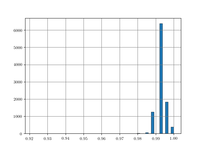
Figure 1: Distance histograms corresponding to the $L_p$ distances between two training examples from different classes. Results obtained on $10000$ training examples of each dataset.
An easy approach to obtain rough "upper bounds" on reasonable $L_p$ adversarial examples is to empirically compute the $L_p$ distance between examples from different classes. For example, this can be done on the training set. Figure 1, for MNIST, Fashion-MNIST, SVHN and Cifar10, shows histograms of the distances $\|x_i - x_j\|_p$ for $y_i \neq y_j$ with $(x_i, y_i)$ being pairs of examples and labels. As can be seen, these distances usually follow a Gaussian-like distribution. For some datasets and $L_p$ norms, the tail towards zero distance is quite short. For example, on Cifar10 for the $L_2$ norm, the distance quickly increases starting at around $3.8$. This means that there is a distance threshold beyond which we suddenly find many examples of different classes within a potential $\epsilon$ ball for $L_p$-constrained adversarial examples. For the $L_\infty$ norm (on Cifar10), in contrast, the tail is significantly longer, starting roughly at $0.26$ and only slowly increasing towards $0.4$. This means that it is still unlikely to find two examples with different class in the $L_\infty$-ball of size $\epsilon = 0.3$.
The obtained upper bounds, computed on $10000$ training examples, are summarized in Table 1. Considering the $L_2$ and $L_1$ norms, some of the obtained upper bounds are already close to $\epsilon$-values used in the literature. For example, in [], I evaluated against $L_2$ adversarial examples with $\epsilon = 3$. However, above $3.23$, label constancy cannot be ensured anymore. Related work [][] uses $\epsilon = 2$ or $\epsilon = 1.5$. For Fashion-MNIST, the upper bound of $1.66$ would prevent such values for $\epsilon$ even though MNIST and Fashion-MNIST are often evaluated using similar hyper-parameters. It can also be seen, that the images of Fashion-MNIST are less binary. Similarly, for SVHN, $\epsilon$ values larger than $2$ for the $L_2$ norm are not meaningful. However, especially for the $L_\infty$ norm, these upper bounds are quite loose in terms of label constancy as I will discuss in the next section.
Table 1: The minimum $L_p$ distance between two examples of different classes for each dataset and $p \in \{\infty, 1, 2\}$ among $10000$ training examples.
| Metric | MNIST | Fashion-MNIST | SVHN | Cifar10 |
|---|---|---|---|---|
| $L_\infty$ | 0.92 | 0.38 | 0.12 | 0.26 |
| $L_1$ | 20.96 | 20.5 | 75.39 | 65.86 |
| $L_2$ | 3.24 | 1.66 | 2.01 | 3.81 |
Visualizing Noise Levels
On MNIST, an $L_\infty$ distance of $0.92$ can be tolerated before "hitting" a training example with different class. Obviously this does not mean that $\epsilon = 0.9$ for $L_\infty$ adversarial examples makes sense: with $\epsilon = 0.5$ any image can be changed to be completely gray, assuming images in $[0,1]$. Thus, Figure 2 shows qualitative examples corresponding to two simple experiments: adding uniform random noise within an $L_p$ ball of size $\epsilon$ and projecting another training example (with different class) onto the $L_p$ $\epsilon$-ball. For example, using $\epsilon = 0.6$ for random $L_\infty$ noise, the digits on MNIST are preserved quite well. The same holds for random noise on all datasets. However, when "blending" images from different classes, this changes. Here, for the left-most image, I considered the $L_p$-ball of size $\epsilon$ around it and projected the right-most image onto this ball. Note that the middle image remains unchanged. It becomes apparent that changes in the $L_\infty$ norm are intuitive, while $L_2$ and $L_1$ changes are less predictable. Even for small values of $\epsilon$, images easily become unrecognizable — meaning they do not clearly belong to any of the classes. This illustrates the problem of evaluating against or training on adversarial examples with large $\epsilon$-constraint: the $\epsilon$-balls might contain "rubbish" images, not belonging to any class.

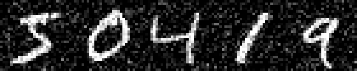


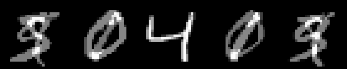


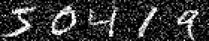


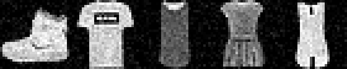
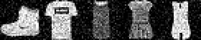
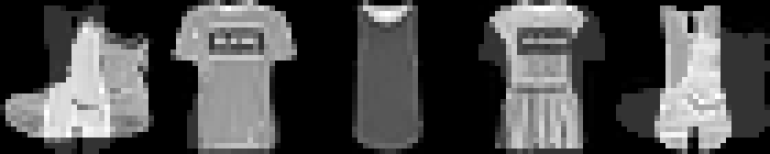
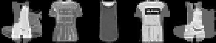

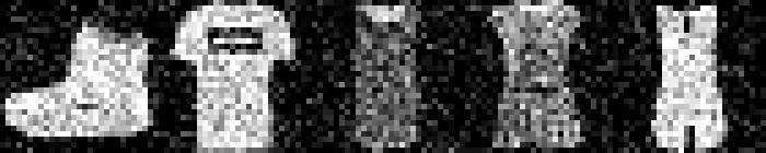
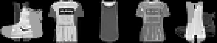

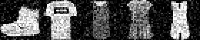
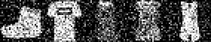
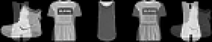
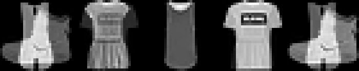


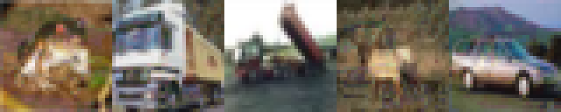
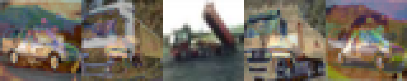
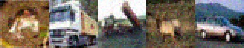
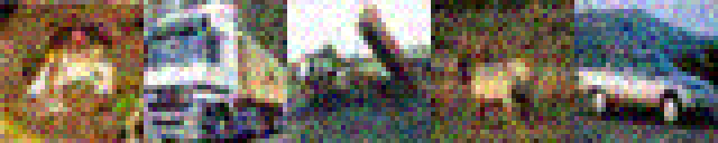
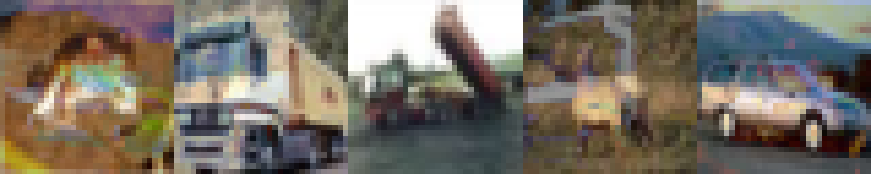
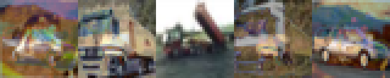
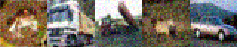
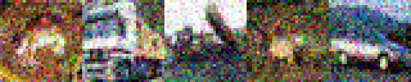

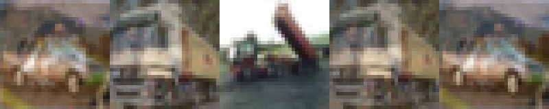
Figure 2: For each dataset and two $\epsilon$ values per $L_p$ norm, I show the following examples. Top: uniform random $L_p$ noise added to five test images. Bottomm: The (second) left-most image projected onto the (second) right-most image. Note that the middle image remains unchanged as reference. As result, for larger $\epsilon$, two different concepts can be seen within the same image. This is most pronounced on MNIST.
Conclusion
Overall, these experiments illustrate the problem of using simple $L_p$ norms as proxy for label constancy or human perception. Furthermore, the results can be used as sanity checks for reviewing or working on adversarial examples. Also, the results show that robustness against arbitrarily large $\epsilon$-balls is not meaningful.
- [] Szegedy, Christian et al. “Intriguing properties of neural networks.” CoRR abs/1312.6199 (2014).
- [] Y. LeCun, L. Bottou, Y. Bengio, and P. Haffner. "Gradient-based learning applied to document recognition." Proceedings of the IEEE, 86(11):2278-2324, November 1998.
- [] Han Xiao, Kashif Rasul, Roland Vollgraf: Fashion-MNIST: a Novel Image Dataset for Benchmarking Machine Learning Algorithms. CoRR abs/1708.07747 (2017).
- [] Yuval Netzer, Tao Wang, Adam Coates, Alessandro Bissacco, Bo Wu, Andrew Y. Ng Reading Digits in Natural Images with Unsupervised Feature Learning NIPS Workshop on Deep Learning and Unsupervised Feature Learning 2011.
- [] Stutz, David et al. “Confidence-Calibrated Adversarial Training: Generalizing to Unseen Attacks.” arXiv: Learning (2019).
- [] Maini, Pratyush et al. “Adversarial Robustness Against the Union of Multiple Perturbation Models.” ArXiv abs/1909.04068 (2019).
- [] Tramèr, Florian and Dan Boneh. “Adversarial Training and Robustness for Multiple Perturbations.” ArXiv abs/1904.13000 (2019).