In general, a variational auto-encoder [] is an implementation of the more general continuous latent variable model. While I used variational auto-encoders to learn a latent space of shapes, they have a wide range of applications — including image, video or shape generation. With this article, I want to start a small series on variational auto-encoders; this article starts discussing the mathematical background of variational inference and variational auto-encoders. However, other parts of the series will cover topics including:

• Denoising variational auto-encoders [];
• Variational auto-encoders with discrete latent space (i.e. categorical/Bernoulli latent variables) [][];
• 2D and 3D Torch implementations of variational auto-encoders including practical tips;

Take a seat and — depending on your background — roughly 30 minutes and I will introduce you to the mathematical framework of variational inference and variational auto-encoders.

Prerequisites. This article is not too heavy on mathematics; however, basic probability theory and linear algebra is necessary for a deeper understanding - including conditional probability, Gaussian distributions, Bernoulli distributions and expectations. Furthermore, the article assumes a basic understanding of (convolutional) neural networks and network training; terms such as cross entropy error or convolutional layers should not be new.

To get a basic understanding of (convolutional) neural networks, have a look at my seminar papers:

• Introduction to Neural Networks;
• Understanding Convolutional Neural Networks.

Overview

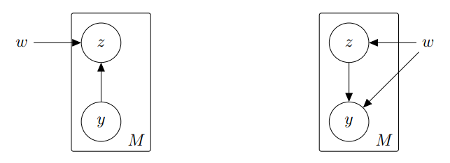
In general, a continuous latent variable model is intended to learn a latent space $\mathcal{Z} = \mathbb{R}^Q$ using a given set of samples $\{y_m\} \subseteq \mathcal{Y} = \mathbb{R}^R$ where $Q \ll R$, i.e. a dimensionality reduction. The model consists of two components which are summarized using the graphical models shown in Figure 1. In particular, the model consists of the generative model $p(y | z)$ given a fixed prior $p(z)$, and the recognition (inference) model $q(z | y)$. For simple Gaussian models, the recognition model $q(z | y)$ as well as the so-called marginal likelihood

$p(y) = \int p(y, z) dz = \int p(y | z)p(z) dz$(1)

can usually be determined and maximized analytically, e.g. for probabilistic Principal Component Analysis (PCA) []. In the case of variational auto-encoders, both the generative and the recognition model are implemented using neural networks. Then, the recognition model as well as the marginal likelihood can only be approximated -- mainly because the integral in Equation (1) becomes intractable. We are going to follow [] and [] to introduce the framework of variational inference which allows to maximize a lower bound on the likelihood.

Variational Inference

In general, variational inference is posed as the problem of finding a model distribution $q(z)$ to approximate the true posterior $p(z | y)$

$q(z) = \arg\min_{q} \text{KL}(q(z) | p(z | y))$(2)

where the Kullback-Leibler divergence $\text{KL}$ is a distance measure defined on probability distributions. The Kullback-Leibler divergence can then be rewritten to obtain a lower bound on the intractable marginal likelihood $p(y)$. The Kullback-Leibler divergence is formally defined as:

A close look at the Kullback-Leibler divergence reveals that the optimization problem in Equation (2) involves computing the marginal likelihood:

$\text{KL}(q(z) | p(z|y)) = \mathbb{E}_{q(z)}\left[\ln\frac{q(z)}{p(z|y)}\right]$

$= \mathbb{E}_{q(z)}[\ln q(z)] - \mathbb{E}_{q(z)}[\ln p(z|y)]$

$= \mathbb{E}_{q(z)}[\ln q(z)] - \mathbb{E}_{q(z)}[\ln p(z,y)] + \ln p(y)$.

Re-arranging left- and right-hand side leads to the evidence lower bound which is also referred to as variational lower bound:

$\ln p(y) = \text{KL}(q(z) | p(z|y)) - \mathbb{E}_{q(z)}[\ln q(z)] + \mathbb{E}_{q(z)}[\ln p(z,y)]$

$\geq - \mathbb{E}_{q(z)}[\ln q(z)] + \mathbb{E}_{q(z)}[\ln p(z,y)]$

$= - \mathbb{E}_{q(z)}[\ln q(z)] + \mathbb{E}_{q(z)}[\ln p(z)] + \mathbb{E}_{q(z)}[\ln p(y|z)]$

$= - \text{KL}(q(z) | p(z)) + \mathbb{E}_{q(z)}[\ln p(y|z)]$

The original problem of maximizing the intractable marginal likelihood $p(y)$ in Equation (1) is then approximated by maximizing the evidence lower bound which we formally define as:

In this general formulation of the evidence lower bound, the model distribution $q(z)$ can be arbitrary. However, in the context of latent variable models, it makes sense to make the model distribution depend on $y$ explicitly, i.e. $q(z | y)$, as we want to be able to reconstruct any $y$ from the corresponding latent code $z$. Then, the evidence lower bound in Equation (3) takes the form of an auto-encoder where $q(z | y)$ represents the encoder and $p(y | z)$ the decoder. Thus, a variational auto-encoder can be trained by maximizing the right-hand-side of Equation (3) after choosing suitable parameterizations for the distributions $p(z)$ and $q(z | y)$. In the following, we discuss the Gaussian case. I leave the discrete case, e.g. the Bernoulli case for a later article.

Gaussian Variational Auto-Encoder

In the framework of variational auto-encoders, the model distribution $q(z|y)$ is implemented as neural network; similarly, in the case of Gaussian variational auto-encoders, both $q(z|x)$ and $p(z)$ are assumed to be Gaussian, specifically

$q(z|y) = \mathcal{N}(z; \mu(y;w), \text{diag}(\sigma^2(y;w)))$

$p(z) = \mathcal{N}(z; 0, I_Q)$

where the dependence on the neural network weights $w$ is made explicit; i.e. both the mean $\mu(y;w) \in \mathbb{R}^Q$ and the (diagonal) covariance matrix $\text{diag}(\sigma^2(y;w)) \in\mathbb{R}^{Q \times Q}$ are predicted using a neural network with parameters $w$ that are to be optimized. Here, $I_Q \in \mathbb{R}^{Q \times Q}$ denotes the identity matrix and $\mathcal{N}$ refers to the Gaussian distribution. In the following we will neglect the weights $w$ for brevity.

Considering the evidence lower bound from Equation (3), i.e.

(3)$ = - \text{KL}(q(z|y)|p(z)) + \mathbb{E}_{q(z|y)}[\ln p(y|z)]$

the Kullback-Leibler divergence between $q(z|y)$ and $p(z)$ can be computed analytically. However, differentiating the lower bound with respect to the hidden weights in $q(z|y)$ is problematic. A classical Monte-Carlo approximation of the expectation $\mathbb{E}_{q(z|y)}[\ln p(y|z)]$ would require differentiating through the sampling process $z \sim q(z | y)$. Therefore, Kingma and Welling [] proposed the so-called reparameterization trick. In particular, the random variable $z \sim q(z|y)$ is reparameterized using a differentiable transformation $g(z, \epsilon)$ based on an auxiliary variable $\epsilon$ drawn from a unit Gaussian:

$z_i = g_i(y, \epsilon_i) = \mu_i(y) + \epsilon_i \sigma_i^2(y)$(4)

with $\epsilon_i \sim \mathcal{N}(\epsilon; 0, 1)$. Overall, given a sample $y_m \in \mathbb{R}^R$, the objective to be minimized has the form

$\mathcal{L}_{\text{VAE}} (w) = \text{KL}(q(z|y_m) | p(z)) - \frac{1}{L}\sum_{l = 1}^L \ln p(y_m | z_{l,m})$

where $z_{l,m} = g(\epsilon_{l,m}, y)$ and $\epsilon_{l,m} \sim \mathcal{N}(\epsilon ; 0, I_Q)$. Here, $L$ is the number of samples to use for the Monte Carlo estimator of the reconstruction error. In practice, the loss $\mathcal{L}_{\text{VAE}}$ is applied on mini-batches and $L = 1$ is usually sufficient.

Given the neural network weights $w$, the generation process can be summarized as follows: draw $z \sim p(z) = \mathcal{N}(z ; 0,I_Q)$, and draw $y \sim p(y|z)$. Similarly, recognition is performed by drawing $z \sim q(z|y)$, i.e. $\epsilon \sim \mathcal{N}(\epsilon ; 0,I_Q)$ and $z = g(y,\epsilon)$. For evaluation purposes, i.e. for measuring the recognition performance, $z$ is usually set to $z = \mathbb{E}_{q(z|y)}[z]$; this can be accomplished by directly considering $\mu(y)$.

Practical Considerations

As mentioned above, the Kullback-Leibler divergence of two Gaussian distributions can easily be calculated directly. As we consider diagonal covariance matrices the Kullback-Leibler divergence is separable over $1 \leq i \leq Q$. Then, we have (see [])

$\text{KL}(\mathcal{N}(z_i ; \mu_{1,i}, \sigma_{1,i}^2)|\mathcal{N}(z_i ; \mu_{2,i},\sigma_{2,i}^2)) = \frac{1}{2} \ln\frac{\sigma_{2,i}}{\sigma_{1,i}} + \frac{\sigma_{1,i}^2}{2\sigma_{2,i}^2} + \frac{(\mu_{1,i} - \mu_{2,i})^2}{2 \sigma_{2,i}^2} - \frac{1}{2}.$

and with $\sigma_{2,i} = 1$ and $\mu_{2,i} = 0$ (and for simplicity $\sigma_i^2 := \sigma_i^2(y) = \sigma_{1,i}^2$ and $\mu_i := \mu_i(y) = \mu_{1,i} $) it follows:

$\text{KL}(p(z_i | y) | p(z_i)) = - \frac{1}{2} \ln \sigma_i + \frac{1}{2} \sigma_i^2 + \frac{1}{2} \mu_i^2 - \frac{1}{2}$.

The remaining part of the objective is the reconstruction error, i.e. the negative log-likelihood $- \ln p(y | z_l)$. This depends on how $p(y|z)$ is modeled; for images or volumes, for example, $p(y | z)$ might decompose over pixels/voxels (where we assume the $R$ to be the dimensionality of the vectorized image/volume):

$p(y|z) = \prod_{i = 1}^R p(y_i | z)\quad\Rightarrow\quad -\ln p(y | z) = -\sum_{i = 1}^R \ln p(y_i | z)$

For binary images or volumes, $p(y_i | z)$ can be modeled as Bernoulli distribution, i.e. $p(y_i | z) = \text{Ber}(y_i ; \theta_i(z))$ where $\theta_i(z)$ is the probability of a pixel/voxel being $1$. These probabilities are directly predicted by the decoder. The negative log-likelihood then reduces to the binary cross entropy error. Otherwise, for continuous output, for example color per pixel/voxel, Gaussian distributions can be used, i.e. $p(y_i | z) = \mathcal{N}(y_i; \mu_i(z), \sigma^2)$ where the $\mu_i(z)$'s are predicted by the decoder and the variance $\sigma^2$ is fixed. In this case, the negative log-likelihood leads to the sum-of-squared error.

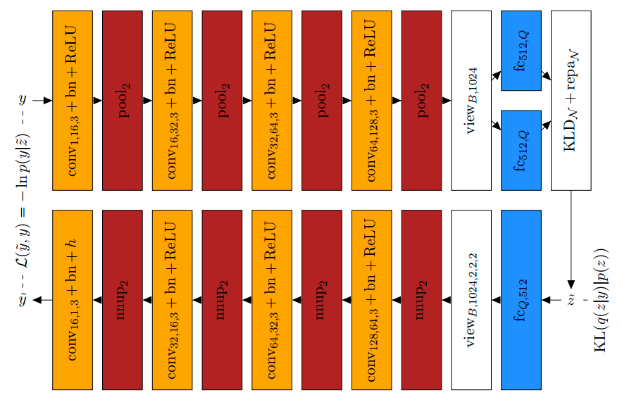
A possible implementation of a variational auto-encoder is shown in Figure 2. Here, the Kullback-Leibler divergence is implemented as layer denoted $\text{KLD}$ and essentially computes the divergence and adds the corresponding derivatives to the gradient flow in the backward pass. Similarly, the reparameterization layer denoted as $\text{repa}$ implements Equation (4).

In practice, letting the encoder predict $\sigma^2(y)$ directly is problematic as the variance $\sigma^2(y)$ may not be negative. Therefore, we can let the encoder predict log-variances instead, i.e. $l_i (y) := \ln \sigma^2(y)$. This makes sure that the variance $\sigma^2(y) = \exp(l_i (y))$ will always be positive. The Kullback-Leibler divergence and the corresponding derivative with respect to $l_i (y)$ as well as the reparameterization trick are easily adapted.

Training a Gaussian variational auto-encoder in practice means balancing the -- possibly conflicting -- objectives corresponding to reconstruction loss and Kullback-Leibler divergence. While the reconstruction loss is intuitively interpretable, e.g. as binary cross entropy error or scaled sum-of-squared error in the Bernoulli and Gaussian cases, respectively, the Kullback-Leibler divergence is less intuitive. Therefore, it might be beneficial to monitor the latent space statistics over a held-out validation set. Concretely, this means monitoring the first two moments of the predicted means, i.e.

$\overline{\mu} = \frac{1}{QM'} \sum_{i = 1}^Q\sum_{m = 1}^{M'} \mu_i(y_m)$

and

$\text{Var}[\mu] = \frac{1}{QM'}\sum_{i = 1}^Q\sum_{m = 1}^{M'} (\mu_i(y_m) - \overline{\mu})^2$

where $M'$ is the size of the validation set. Additionally, it is worth monitoring the first moment of the predicted log-variances

$\overline{l} = \frac{1}{QM'} \sum_{i = 1}^Q\sum_{m = 1}^{M'} \ln \sigma_i^2(y_m) = \frac{1}{QM'} \sum_{i = 1}^Q\sum_{m = 1}^{M'} l_i(y_m).$

Note that these statistics are computed over all $Q$ dimensions of the latent space -- this is appropriate as the prior $p(z)$ is a unit Gaussian such that all dimensions can be treated equally. During training, these statistics should converge to a unit Gaussian, i.e. $\overline{\mu} \approx 0$ and $\text{Var}[\mu] \approx 1$, and the network should be capable of making certain predictions, i.e. small $\overline{l}$.

Outlook

The next two articles will cover two interesting extensions of vanilla variational auto-encoders as introduced in []:

• Denoising variational auto-encoders [];
• and variational auto-encoders with categorical/Bernoulli latent variables [][].

Afterwards, we will discuss implementations and practical tips in Torch.

• [] D. M. Blei, A. Kucukelbir, and J. D. McAuliffe. Variational inference: A review for statisticians. CoRR, abs/1601.00670, 2016.
• [] C. Doersch. Tutorial on variational autoencoders. CoRR, abs/1606.05908, 2016.
• [] D. P. Kingma and M. Welling. Auto-encoding variational bayes. CoRR, abs/1312.6114, 2013.
• [] S. Kullback. Information Theory and Statistics. Wiley, New York, 1959.
• [] M. E. Tipping and C. M. Bishop. Probabilistic principal component analysis. Journal of the Royal Statistical Society, Series B, 61:611-622, 1999.
• [] D. J. Im, S. Ahn, R. Memisevic, and Y. Bengio. Denoising criterion for variational auto-encoding framework. In AAAI Conference on Artificial Intelligence, pages 2059-2065, 2017.
• [] E. Jang, S. Gu, and B. Poole. Categorical reparameterization with gumbel-softmax. CoRR, abs/1611.01144, 2016.
• [] C. J. Maddison, A. Mnih, and Y. W. Teh. The concrete distribution: A continuous relaxation of discrete random variables. CoRR, abs/1611.00712, 2016.