iPiano is an iterative optimization algorithm combining forward-backward splitting with an inertial force to tackle the problem
$\min_{x \in \mathbb{R}^n} h(x) = \min_{\mathbb{R}^n} f(x) + g(x)$.(1)
Here, $f$ is required to be differentiable, but might be non-convex, while $h$ is required to be convex, but might be non-differentiable.
This article discusses iPiano in more detail and presents an implementation which was written as part of a seminar on "Selected Topics in Image Processing" advised by Prof. Berkels at RWTH Aachen University. The implementation is available on GitHub:
iPiano on GitHubThe corresponding seminar paper will follow soon!
Background
Let $g$ be a proper, convex and lower semi-continuous such that the proximal mapping
$\text{prox}_{\alpha g} (x) := \arg\min_{\hat{x}} g(\hat{x}) + \frac{1}{2\alpha} \|x - \hat{x}\|_2^2$
is well-defined (i.e. there exists a unique solution to the above minimization problem). Furthermore, let $\partial g$ be the subdifferential of $g$, defined as
$\partial g (x) := \{w \in \mathbb{R}^n | g(x) + w^T(\hat{x} - x) \leq g(\hat{x}) \forall \hat{x}\in \mathbb{R}^n\}$.
Then, using $\partial h(x) = \nabla f(x) + \partial g(x)$, the first-order optimality condition for Equation (1) is
$0 \in \partial h(x) \quad\Leftrightarrow\quad - \nabla f(x) \in \partial g(x)$.
From this optimality condition, it can be derived that the following fixpoint equation gives a solution to Equation (1):
$x^\ast = \text{prox}_{\alpha g} (x^\ast - \alpha \nabla f(x^\ast))$
which motivates the forward-backward splitting algorithms as for example discussed in detail in [1]. The underlying iterative scheme of forward-backward splitting is
$x^{(n + 1)} = \text{prox}_{\alpha_n g} (x^{(n)} - \alpha_n \nabla f(x^{(n)}))$
where $\alpha_n$ is the step size in the $n$-th iteration and $x^{(n)}$ the $n$-th iterate. Considering an inertial force (i.e. a momentum term), this scheme can be extended as follows:
$x^{(n + 1)} = \text{prox}_{\alpha_n g} (x^{(n)} - \alpha_n \nabla f(x^{(n)}) + \beta_n (x^{(n)} - x^{(n - 1)})$(2)
where $\beta_n$ is the momentum parameter in the $n$-th iteration. Equation (2) is the basis of the iPiano algorithm proposed by Ochs et al. [1]. Obviously, the key lies in choosing appropriate $\alpha_n$ and $\beta_n$ in order to guarantee convergence.
iPiano and Variants
In the following, we discuss some variants of the iterative scheme in Equation (2).
ciPiano. Both the step size parameter $\alpha_n$ as well as the momentum parameter $\beta_n$ can be chosen to be constant, see Algorithm 1.
function constant_step_forward_backward(
        $g$, $f$,
        $L$ // Lipschitz constant of $\nabla f$
    )
    choose $\beta \in [0, 1)$
    choose $\alpha < \frac{2(1 - \beta)}{L}$
    initialize $x^{(0)}$
    for $n = 1,\ldots$
        $x^{(n + 1)} = \text{prox}_{\alpha g} (x^{(n)} - \alpha \nabla f(x^{(n)}) + \beta(x^{(n)} - x^{(n - 1)}))$
Algorithm 1 (ciPiano): iPiano with constant step size and momentum parameter.
nmiPiano. In order to choose $\alpha_n$ appropriately, the Lipschitz constant $L$ needs to be known (or estimated). nmiPiano, presented in Algorithm 2, uses backtracking to estimate $L$ locally in each iteration. In particular, given $x^{(n)}$ and $x^{(n + 1)}$, the estimate $L_n$ is required to satisfy
$f(x^{(n + 1)}) \leq f(x^{(n)}) + \nabla f(x^{(n)})^T(x^{(n + 1)} - x^{(n)}) + \frac{L_n}{2}\|x^{(n + 1)} - x^{(n)}\|_2^2$.(3)
In practice, $x^{(n + 1)}$ is re-estimated until a$L_n \in \{L_{n - 1}, \eta L_{n - 1}, \eta^2 L_{n - 1}, \ldots \}$
is found satisfying Equation (3). nmiPiano adapts $\alpha_n$ according to the estimated $L_n$ while keeping $\beta_n$ fixed.
function constant_step_forward_backward(
        $g$, $f$,
        $L$ // Lipschitz constant of $\nabla f$
    )
    choose $\beta \in [0, 1)$
    choose $L_{- 1} > 0$
    choose $\eta > 1$
    initialize $x^{(0)}$
    for $n = 1,\ldots$
        $L_n := \frac{1}{\eta} L_{n - 1}$ // Initial estimate of $L_n$
        repeat
            $L_n := \eta L_n$ // Next estimate of $L_n$
            choose $\alpha_n < \frac{2(1 - \beta)}{L_n}$
            $\hat{x}^{(n + 1)} = \text{prox}_{\alpha_n g} (x^{(n)} - \alpha_n \nabla f(x^{(n)}) + \beta (x^{(n)} - x^{(n - 1)}))$
        until (3) is satisfied with $\hat{x}^{(n + 1)}$
        $x^{(n + 1)} := \hat{x}^{(n + 1)}$
Algorithm 2 (nmiPiano): iPiano with constant momentum parameter.
iPiano. Algorithm 3, called iPiano, adapts both $\alpha_n$ and $\beta_n$ based on the current estimate $L_n$ of the local Lipschitz constant. Additionally, auxiliary variables $\delta_n$, $\gamma_n$ and constants $c_1$, $c_2$ (close to zero) are introduced in order to bound suitable $\alpha_n$ and $\beta_n$. Specifically, $\alpha_n \geq c_1$ and $\beta_n$ are chosen such that
$\delta_n := \frac{1}{\alpha_n} - \frac{L_n}{2} - \frac{\beta_n}{2\alpha_n} \geq \gamma_n := \frac{1}{\alpha_n} - \frac{L_n}{2} - \frac{\beta_n}{\alpha_n} \geq c_2$.
Then, it can be shown that $\delta_n$ is monotonically decreasing. This, in turn, is required to prove convergence, see [1] for details.
function constant_step_forward_backward(
        $g$, $f$,
        $L$ // Lipschitz constant of $\nabla f$
    )
    choose $L_{- 1} > 0$
    choose $\eta > 1$
    initialize $x^{(0)}$
    for $n = 1,\ldots$
        $L_n := \frac{1}{\eta} L_{n - 1}$ // Initial estimate of $L_n$
        repeat
            $L_n := \eta L_n$ // Next estimate of $L_n$
            repeat
                choose $\alpha_n \geq c_1$
                choose $\beta_n \geq 0$
                $\delta_n := \frac{1}{\alpha_n} - \frac{L_n}{2} - \frac{\beta_n}{2\alpha_n}$
                $\gamma_n := \frac{1}{\alpha_n} - \frac{L_n}{2} - \frac{\beta_n}{\alpha_n}$
            until $\delta_n \geq \gamma_n \geq c_2$
            $\hat{x}^{(n + 1)} = \text{prox}_{\alpha_n g} (x^{(n)} - \alpha_n \nabla f(x^{(n)}) + \beta_n (x^{(n)} - x^{(n - 1)}))$
        until (3) is satisfied with $\hat{x}^{(n + 1)}$
        $x^{(n + 1)} := \hat{x}^{(n + 1)}$
Algorithm 3 (iPiano): iPiano.
Implementation
Building. The implementation is based on Eigen, OpenCV, GLog and Boost and may be built using CMake:
git clone https://github.com/davidstutz/ipiano
cd ipiano
mkdir build
cd build
cmake ..
make
Usage. The following example illustrates usage on a simple one-dimensional signal denoising application. In particular, given a noisy signal $u^{(0)}\in \mathbb{R}^n$, we minimize
$h(u; u^{(0)}, \lambda) = \underbrace{\sum_{i = 1}^n \rho_1(u_i - u^{(0)}_i)}_{=g(u;u^{(0)})} + \lambda \underbrace{\left[\sum_{n = 2}^n \rho_2(u_i - u_{i - 1})\right]}_{=f(u)}$(4).
We choose
$\rho_1(x) = |x|$ and $\rho_2(x; \sigma) = \log\left(1 + \frac{x^2}{\sigma^2}\right)$
such that $g(u; u^{(0)})$ is convex but not differentiable, while $f(u)$ is differentiable but not convex.
This problem is solved using the following code snippet:
// We randomly sample a signal in the form of a Nx1 Eigen matrix:
Eigen::MatrixXf signal;
sampleSignal(signal);

// perturbed_signal is the noisy signal we intend to denoise:
Eigen::MatrixXf perturbed_signal = signal;
perturbSignal(perturbed_signal);

// Basic denoising functionals are provided in functionals.h
// f_forentzianPairwise is a regularizer based on the lorentzian function;
// i.e. it is differentiable but not convex.
// g_absoluteUnary is an absolute data term which is convex but not differentiable.
// The corresponding gradient and proximal mapping are implemented in functionals.h
// and described in detail in [2].
std::function<float(const Eigen::MatrixXf&)> bound_f
        = std::bind(Functionals::Denoising::f_lorentzianPairwise, std::placeholders::_1, sigma, lambda);
std::function<void(const Eigen::MatrixXf&, Eigen::MatrixXf&)> bound_df
        = std::bind(Functionals::Denoising::df_lorentzianPairwise, std::placeholders::_1, std::placeholders::_2, sigma, lambda);
std::function<float(const Eigen::MatrixXf&)> bound_g
        = std::bind(Functionals::Denoising::g_absoluteUnary, std::placeholders::_1, perturbed_signal);
std::function<void(const Eigen::MatrixXf&, Eigen::MatrixXf&, float)> bound_prox_g
        = std::bind(Functionals::Denoising::prox_g_absoluteUnary, std::placeholders::_1, perturbed_signal, std::placeholders::_2, std::placeholders::_3);

// The initial iterate (i.e. starting point) will be a random signal.
Eigen::MatrixXf x_0 = Eigen::MatrixXf::Zero(M, 1);
perturbSignal(x_0);

// nmiPiano provides the following options, see nmipiano.h or the discussion below.
nmiPiano::Options nmi_options;
nmi_options.x_0 = x_0;
nmi_options.max_iter = 1000;
nmi_options.L_0m1 = 100.f;
nmi_options.beta = 0.5;
nmi_options.eta = 1.05;
nmi_options.epsilon = 1e-8;

// Both nmiPiano and iPiano provide callbacks to monitor progress.
// The default_callback writes progress to std::cout, other callbacks to
// write the progress to file are available in nmipiano.h and ipiano.h
std::function<void(const nmiPiano::Iteration &iteration)> nmi_bound_callback
        = std::bind(nmiPiano::default_callback, std::placeholders::_1, 10);

// For initialization, we provide f and g as well as their gradient/proximal mapping,
// and the callback defined above.
nmiPiano nmipiano(bound_f, bound_df, bound_g, bound_prox_g, nmi_options,
        nmi_bound_callback);

// Optimization is done via .optimize expecting two arguments which will be the
// final iterate as well as the corresponding function value (i.e. h = f + g)
Eigen::MatrixXf nmi_x_star;
float nmi_f_x_star;
nmipiano.optimize(nmi_x_star, nmi_f_x_star);
The objective $h$ is provided through its parts: $g$, $f$, $\text{prox}_{\alpha g}$ and $\nabla f$. The parts are provided as function bindings providing the following interfaces:
/** \brief Possibly non-convex but smooth part, i.e. f.
\param[in] x
\return f(x)
 */
static float f(const Eigen::MatrixXf &x);

/** \brief Derivative of f, i.e. \nabla f.
\param[in] x
\param[out] df_x
 */
static void df(const Eigen::MatrixXf &x, Eigen::MatrixXf &df_x);

/** \brief Convex but possibly non-smooth part, i.e. g.
\param[in] x
\return
 */
static float g(const Eigen::MatrixXf &x);

/** \brief Proximal map of g.
\param[in] x
\param[out] prox_f_x
\param[in] alpha
 */
static void prox_g(const Eigen::MatrixXf &x, Eigen::MatrixXf &prox_f_x, float alpha);
In the presented example, additional parameters (e.g. the noisy signal $x^{(0)}$) are bound beforehand, as in the case of $g(x; x^{(0)})$:
std::function<float(const Eigen::MatrixXf&)> bound_g
        = std::bind(Functionals::Denoising::g_absoluteUnary, std::placeholders::_1, perturbed_signal);
The example demonstrates the usage of nmiPiano, i.e. Algorithm 2. The provided options are summarized below:
nmi_options.x_0: the initial iterate;nmi_options.max_iter: maximum number of iterations;nmi_options.beta: fixed $\beta$, i.e. the parameter governing the momentum term/inertial force;nmi_options.eta: parameter for backtracking to find the local Lipschitz-constant L_n in each iteration, see Equation (3);nmi_options.L_0m1: initial estimate of the local Lipschitz-constant; during initialization, the local Lipschitz-constant is estimated aroundnmi_options.x_0and the maximum of the estimate andnmi_options.L_0m1is taken;nmi_options.epsilon: stopping criterion; if epsilon is greater than zero, iterations stop if the squared norm of the difference of two consecutive iterates is smaller than epsilon.
A usage example for iPiano, i.e. Algorithm 1, can be found in the repository.
Results
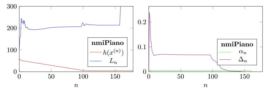
Figure 1 shows the convergence of nmiPiano for $\beta_n = 0.5$. The initial local Lipschitz constant is set to $L_{-1} = 100$ (i.e. nmi_options.L_0m1); in practice, this may be necessary to guarantee (or speed up) convergence. As can be seen, the initial $L_{-1} = 100$ is not far from the estimated $L_n \approx 200$ until the algorithm converges.
Qualitative results are shown in Figure 2, where we consider both
$\rho_{1,\text{abs}}(x) = |x|$ and $\rho_{1,\text{sqr}}(x) = x^2$.
