Ian Goodfellow's Deep Learning textbook quickly became a standard for generations to come. Although I was introduced to most of the cencepts a few years earlier — mainly through seminars at RWTH Aachen University —, I still took the chance and read most of the chapters. In this article, I want to present some of my notes I took while reading the textbook. Note that an online version of the book is available here.
As I was familiar with the basics of machine learning and feed-forward neural networks, I started with chapter 7. Additionally, I skipped chapters 12, 13 and 14 as they are of less interest for me.
Chapter Notes
Click on a chapter to open the corresponding notes.
In chapter 7, Goodfellow et al. discuss several regularization techniques for deep learning in detail, and give valuable interpretations and relationships between them. They also revisit the goal of regularization. In particular, they characterize regularization as an approach to trade increased bias for reduced variance. The ultimate goal is to take a model where variance dominates the error (e.g. overfitted models) and reduce the variance in the hope to only slightly increase the bias. In the following, some regularization techniques are discussed, focussing on the practical insights provided by Goodfellow et al. instead of describing the techniques in detail.
Norm regularization ($L_2$ and $L_1$ regularization). Usually only the weights are regularized, not the biases. Therefore, it might also be interesting to regularize the weights in different layers differently strong. Two useful interpretations of $L_2$ regularization are the following:
- $L_2$ regularization shrinks the weights during training. However, Goodfellow et al. also show that components of the weights that correspond to directions that do not contribute to reducing the cost are decayed away faster than more useful directions. This is the result of the analysis of the eigenvectors and eigenvalues of the Hessian matrix (assuming a local, quadratic and convex approximation of the cost function).
- Using $L_2$ regularization, the training set is perceived to have higher variance. As a result, weight components corresponding to features that have low covariance with the target output compared to the perceived variance shrink faster.
Data augmentation. Goodfellow et al. briefly discuss the importance and influence of data augmentation to increase the size of the training set. Unfortunately, they give little concrete examples or references on this topic. They mostly focus on adding noise to either the input units or the hidden units. In a separate section on noise robustness, they also discuss the possibility to add noise to the weights in order to make the final model more robust to noise. Later this topic is also related to adversarial training, where training samples are constructed to "fool" the network while being similar to existing training samples. Here, as well, they do not give many concrete examples.
Early stopping. Beneath discussing the interpretation of early stopping as regularizer, Goodfellow et al. also focus on the problem utilizing early stopping while still being able to train on the full training set (as early stopping requires a part of the training set as validation set). The first approach discussed involves retraining the model on the full training set and training for approximately as many iterations as before when training with early stopping. The second approach fine-tunes the model on the full training set and stops when the training error reaches the training error when training was stopped using early stopping.
Dropout. Goodfellow et al. discuss the two important interpretations: dropout as bagging, and dropout as regularizer. In the first case, the most valuable insight provided is how to get the advantage of training with dropout at testing time, i.e. how to approximate the ensemble prediction.
In chapter 8, Goodfellow et al. discuss optimization for deep neural networks. In particular, they focus on three different aspects:
- How learning differs from classical optimization;
- Why learning deep neural networks is difficult;
- And concrete optimization techniques (both "fixed" learning rate and adaptive learning rate) as well as parameter initialization schemes.
How learning differs from classical optimization. One of the most important difference between learning and optimization is that learning tries to indirectly optimize a (usually) intractable measure while for optimization the goal is to directly optimize the objective at hand. In learning, the overall goal is to minimize the expected generalization error, i.e. the risk. However, as the generating distribution is usually unknown (and/or intractable), the empirical risk on a given training set is minimized instead. Furthermore, in learning, the empirical risk is usually not minimized directly, for example if the loss is not differentiable. Instead, a surrogate loss is minimized and optimization is usually stopped early to prevent overfitting and improve generalization. This is in contrast to classical optimization where the objective is usually not replaced by a surrogate objective. Lastly, in learning the optimization problem can usually be decomposed as a sum over the training samples.
Due to computational limits and considerations regarding generalization and implementation, researchers have early argued about so-called stochastic (mini-batch) optimization schemes. This discussion is usually specific to the task of learning and cannot be generalized to classical optimization. Some of the arguments made by Goodfellow et al. are summarized in the following points:
- The standard error of a mean estimator is $\frac{\sigma}{\sqrt{n}}$ where $\sigma$ is the true standard deviation and $n$ the number of samples. Thus, there is less than linear returns in using more samples for estimating statistics (e.g. the gradient).
- Small batches can offer regularization effects due to the introduced noise. However, this usually requires a smaller learning rate and induces slow learning.
Why learning deep neural networks is difficult. Goodfellow et al. discuss several well-known problems when training deep neural networks. However, they also give valuable insights of how these problems are related and approached in practice. The obvious argument is that used optimization techniques assume access to the true required statistics, such as the true gradient. However, in practice, the gradient is noisy and usually estimated based on stochastic mini-batches. Furthermore, the problem can be ill-conditioned, i.e. the corresponding Hessian matrix may be ill-conditioned. Goodfellow et al. provide an intuitive explanation based on a second-order Taylor expansion of the gradient descent update. Then, it can easily be shown that a gradient descent update of $-\epsilon g$, with $g$ begin the gradient, adds $\frac{1}{2} \epsilon^2 g^T H g - \epsilon g^Tg$ to the cost. However, this may get positive. In particular, Goodfellow et al. describe the case that $g^T g$ stays mostly constant during training while $g^T Hg$ may increase by an order of magnitude. They also describe that monitoring both values during training might be beneficial (the former is also useful to detect whether learning has problems with local minima).
Another important discussion provided by Goodfellow et al. is concerned with the importance of local minima and saddle points. The main insight is that in high-dimensional spaces, local minima become rare and saddle points become much more frequent. This can be explained by the corresponding Hessian matrix. For local minima, all eigenvalues need to be positive, while for saddle points, both positive and eigenvalues are present. Obviously, the latter case becomes more frequent in high-dimensional spaces. Furthermore, local minima are much more likely to have low cost. This, too, can be explained by the Hessian being more likely to have only positive eigenvalues in low cost areas. Therefore, in high-dimensional spaces, saddle-points are the more serious problem in learning. Still, both cases induce a difficulty and require optimization methods to be tuned to the specific learning task.
Lastly, Goodfellow et al. discuss the case of cliffs in the energy landscape corresponding to the learning problem. In particular, cliffs refer to extremely steep regions (which may occur suddenly in more or less flat regions). These cliffs usually cause extremely high gradient and may result in large jumps made by the gradient descent update, potentially increasing the cost. However, they also provide a simple counter-measure (see Chapter 11): gradient clipping. Gradient clipping is usually done by either clipping the individual entries of the gradient vector at a maximum value, or clipping the gradient vector as whole at a specific norm. Both approaches seem to work well in practice.
Basic optimization techniques. As basis for the remaining chapters, Goodfellow et al. discuss stochastic gradient descent with momentum as well as Nesterov's accelerated gradient method. Details can be found in the chapter. Especially, the detailed explanation of the momentum term can be recommended.
Some interesting arguments made by Goodfellow et al. concern the convergence rate. It is well known that the convergence rate of stochastic gradient descent in the strictly convex case is $\mathcal{O}\left(\frac{1}{k}\right)$. However, the generalization error cannot be reduced faster than $\mathcal{O}\left(\frac{1}{k}\right)$ such that, from the machine learning perspective, it might not be beneficial to consider algorithms offering faster convergence (as this may correspond to overfitting).Weight initialization schemes. Goodfellow et al. discuss several weight initialization schemes without going into too much details. Instead of looking at the individual schemes, value can be found in the discussed heuristics - especially as they explicitly state that initialization (and optimization) is not well understood yet. The following presents an unordered list detailing some of the discussed heuristics:
- An important aspect of weight initialization is to break symmetry, i.e. units with the same or similar input should have different initial weights as otherwise they would develop very similarly during training. This motivates random initialization using a high-entropy distribution - usually Gaussian or uniform.
- Biases are usually initialized to constant values. In many cases, 0 might be sufficient, however for saturating activation functions or output activation function non-zero initialization should be considered.
- The right balance between large initial weights and not-too-large initial weights is important. While too large weights may cause gradient explosion (if no clipping is used), large weights ensure that activations and errors (in forward and backward pass, respectively) are still numerically significant (i.e. distinct from 0).
- Independent of the initialization scheme used, it is recommended to monitor the activations and gradients of all layers on individual mini-batches. If activations or gradients in specific layers vanish, the scale or range of initialization may need to be adapted.
Adaptive learning rate techniques. Goodfellow et al. discuss several techniques including AdaGrad, Adam and RMSProp (with and without momentum). However, they are not able to answer the question which of the techniques is to be preferred.
Meta algorithms. Finally, Goodfellow et al. discuss a set of meta algorithms to aid optimization. The most interesting part is concerned with batch normalization. In particular, they are able to provide an extremely intuitive motivation. Using any gradient descent based optimization technique, the computed updates for a particular layer assume that preceeding layers do not change - which of course is wrong. They also discuss that batch normalization - through normalizing the first and second moments - implicitly reduces the expressive power of the network, especially when using linear activation functions. This results in the model being easier to train. To avoid the restrictions in expressive power, batch normalization applies a reparameterization to allow non-zero mean and non-unit variance.
In chapter 9, Goodfellow et al. discuss convolutional networks in quite some detail. However, instead of focussing on the technical details, they discuss the high-level interpretations and ideas.
For example, they motivate the convolutional layer by sparse interactions, parameter sharing and equivariant representations. With sparse interactions, they refer to the local receptive field of individual units within convolutional networks (as the used kernels are usually small compared to the input size). Parameter sharing is achieved by using the same kernel at different spatial locations, such that neighboring units use the same weights. In this regard, some of the discussed alternative uses of convolution in neural networks are interesting. For example tiled convolution where different kernels are used for neighboring units by cycling through a fixed number of different kernels. Unshared convolution is also briefly discussed. Finally, equivariant representation refers to the translation invariance of the convolution operation.
Regarding pooling, they focus on the invariance introduced through pooling. However, they do not discuss the different pooling approaches used in practice. Unfortunately, They also don't give recommendations of when to use pooling and which pooling scheme to use. In contrast, they discuss the interpretation of pooling as infinitely strong prior. An interesting interpretation where pooling is assumed to place an infinitely strong prior on units invariant to local variations (like small translations or noise). In the same sense, convolutional layers place an infinitely strong prior on neighboring units having the same weights.
Finally, the importance of random and unsupervised features is briefly discusses. Here, an interesting reference is [1] where it is shown that random features work surprisingly well.
They conclude with a longer discussion of the biological motivation of convolutional networks given by neuroscience. While most of the discussed aspects are well-known, it is an interesting summary of different aspects motivating research in convolutional networks. Some of the main points is to distinguish simple and complex cells, and the simple cells in particular can often be modeled using Gabor filters. Another interesting insight is the low resolution used by the human eye. Only individual locations are available in higher resolution. Unfortunately, Goodfellow et al. do not provide many references how this model of attention can be implemented in modern convolutional networks.
- [1] A. M. Saxe, P. W. Koh, Z. Chen, M. Bhand, B. Suresh, A. Ng. On random weights and unsupervised feature learning. ICML, 2011.
In chapter 11, Goodfellow et al. give an introduction to recurrent neural networks as well as corresponding further developments like long short-term memory networks (LSTM). During their discussion they focus on three different schemes (Goodfellow et al. call it "patterns") of recurrent neural networks (of which the first two schemes are illustrated in Figure 1):
- Recurrent neural networks producing an output at each iteration and the hidden units are connected through time.
- Recurrent neural networks producing an output at each iterations where the output is propagated to the hidden units in the next time step.
- Recurrent neural networks that read a complete sequence and then produce a single output.

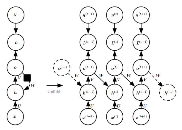
Figure 1 (click to enlarge): Recurrent neural network where the hidden units are propagated through time (left) and where only the output is propagated through time (right). As detailed by Goodfellow et al., the second option represents strictly lower expressiveness in terms of which functions can be modeled.
The key idea that makes recurrent neural networks interesting, is that the parameters (i.e. $W$, $U$, $V$ ...) are shared across time, allowing for variable length sequences to be processed. In addition, parameter sharing is important to generalize to unseen examples of different lengths. The general equations corresponding to the first scheme are as follows:
$a^{(t)} = b + Wh^{(t-1)} + U x^{(t)}$
$h^{(t)} = \text{tanh}(a^{(t)})$
$o^{(t)} = c + Vh^{(t)}$
$\hat{y}^{(t)} = \text{softmax}(o^{(t)})$
Relating to Figure 1, on top of the output $o^{(t)}$ a loss $L^{(t)}$ is applied which implicitly performs the softmax operation to compute $\hat{y}^{(t)}$ and computes the loss with regard to the true output $y^{(t)}$.
Recurrent neural networks are generally trained using error backpropagation through time, which describes error backpropagation applied to the individual networks starting from the last time step and going back to the first time step. As the parameters across time are shared, the gradients with respect to the involved parameters represent sums over time. For example, regarding $W$ the gradient is easily derived (by recursively applying the chain rule) as
$\nabla_W L = \sum_t \sum_i \left(\frac{\partial L}{\partial h_i^{(t)}}\right) \nabla_{W^{(t)}} h_i^{(t)}$
when considering the first model of Figure 1.
While the presented recurrent network is shallow - having only one hidden layer - deep recurrent neural networks can add multiple additional layers. Interestingly, one has many options of how these additional layers are connected through time. Goodfellow et al. illustrate this freedom using Figure 2. Note that the black square indicates a time delay of one time step for unfolding (see chapter 10.1 for details) the model.

Figure 2 (click to enlarge): Examples of possible deep recurrent network architectures.
Towards the end of the chapter, Goodfellow et al. focus on learning long-term dependencies. The described problem corresponds to exploding or vanishing gradients (with respect to time) when training recurrent neural networks for long sequences. Beneath simple techniques such as gradient clipping (also see chapter 8), several model modifications are discussed that simplify learning long-term dependencies. Among these models, Goodfellow et al. also discuss long short-term memory (LSTM) models. Other approaches include skip connections and leaky units.
Chapter 11 is among the most interesting chapters for deep learning practitioners that already have some background on the involved theory and algorithms. What Goodfellow et al. call "Practical Methodology" can best be described as a loose set of tips and tricks for approaching deep learning problems. They give the following, general process that should be followed:
- Define the problem to be solved including metrics used to access whether the problem was solved; it is also beneficial to define expected results in terms of the chosen metrics.
- Get a end-to-end prototype running that includes the selected metric.
- Incrementally do the following: diagnose a component (or aspect) that causes the system to under perform (e.g. hyperparameters, bugs, low-quality data, not enough data, model complexity etc.) and fix it.
Surprisingly, this approach has many parallels with modern, agile software engineering principles (e.g. prototyping, iterative development, risk focus).
Goodfellow et al. then discuss some of these aspects in detail. The most interesting points are made on diagnosing a running end-to-end system:
- Visualize the results: do not focus on the quantitative results in terms of the selected metrics, also visualize the results to asses them qualitatively. This also includes looking at examples that are considered very difficult or very easy.
- Always monitor training and test performance: also discussed in chapter 7, training and test performance may give important clues regarding hyperparameters or regularization such as early stopping. However, it might also help to decide whether bugs cause problems or underfitting/overfitting is a problem.
- Try a tiny dataset: try a smaller or easier training set; this might be helpful to see whether bugs exist.
- Monitor activations and gradients: monitoring the activations may provide clues about the model complexity and activation functions. Together with monitoring the gradients, e.g. the magnitude, might be helpful to asses optimization performance, problems with the hyperparameters etc.
In Chapter 15, Goodfellow et al. consider representation learning, focussing on unsupervised pre-training. Specifically, they discuss when and why unsupervised pre-training may help the subsequent supervised task. The two discussed interpretations are:
- Unsupervised pre-training acts as regularizer by limiting the initial parameters to a specific region in parameter space.
- Unsupervised pre-training helps to learn representation characterizing the input distribution; this may help learning mappings from input to output.
Regarding the first interpretation, it was originally assumed to help optimization by avoiding poor local minima. However, Goodfellow et al. emphasize that it is known by now that local minima aren't a significant problem in deep learning. That may also be one of the reasons why unsupervised pre-training isn't as popular anymore (especially compared to supervised pre-training or various forms of transfer learning). However, unsupervised pre-training may make optimization more deterministic. Goodfellow et al. specifically argue that unsupervised pre-training causes deep learning to consistently reach the same "solution". This suggests that unsupervised pre-training reduces the variance of the learned estimator. It is hard to say when unsupervised pre-training is beneficial when using this interpretation.
The second interpretation gives more clues about when unsupervised pre-training may be beneficial. For example, if the initial representation is poor. Goodfellow et al. name the example of word representations and also argue that there is less benefit for vision tasks as discrete images already represent an appropriate representation of the data. When thinking of unsupervised pre-training (or semi-supervised training) as identifying the underlying causes of the data, success may depend on the causal factors involved and the data distribution. For example, assumptions such as sparsity or independence may or may not be present regarding the causes. Furthermore, from a uniform data distribution, no useful representation can be learned. From a highly multi-modal distribution, unsupervised pre-training may already identify the different modes without knowing the semantics.
Overall, the chapter gives a good, high-level discussion of unsupervised pre-training and representation learning in general without going into algorithmic details. Two important takeaways are the two presented interpretations that can be used to reason about unsupervised pre-training.
In Chapter 16, Goodfellow et al. briefly recap directed and undirected graphical models including d-separation, factor graphs and ancestral sampling. However, I found that there are better textbooks or chapters on graphical models. A similarly brief introduction can be found in [1] and an extensive discussion is available in [2].
In the end, they relate graphical models to deep learning yielding some interesting insights. While traditional graphic models usually have fewer unobserved variables and tend to have sparse connections such that exact inference is possible, the deep learning approach usually focusses on having many hidden, latent variables with dense connections in order to learn distributed representation. Exact inference is usually not expected to be possible and even marginals are not tractable. It is usually sufficient to be able to draw approximate samples and efficiently compute the gradient of the underlying energy function (while the energy itself does not need to be tractable).
Finally, they briefly introduce restricted Boltzmann machines (RBMs) (note that there might be more detailed discussions available). An RBM is an energy-based model with binary hidden and visible variables, $h$ and $v$, respectively:
$E(v,h) = -b^Tv - c^Th - v^TWh$
where $b$, $c$ and $W$ are real-valued parameters that are learned. Note that there is no interaction between any two hidden variables or any two visible variables (as illustrated by the $−b^T v$ and $−c^T h$ terms). Instead, only parts of visible and hidden variables are, usually densely, connected through the weight matrix $W$. The individual conditional distributions are easily computed by:
$P(h_i = 1 | v) = \sigma(v^T W_{i,j} + b_i)$
Overall, this allows for efficient Gibbs sampling. Furthermore, the energy is linear in all of its parameters such that the derivatives are easy to derive.
- [1] C. M. Bishop. Pattern Recognition and Machine Learning. Springer, 2006.
- [2] D. Koller, N. Friedman. Probabilistic Graphical Models: Principles and Techniques. MIT Press, 2009.
In chapter 17, after discussing structured predictions using graphical models in Chapter 16, Goodfellow et al. briefly introduce basic Monte Carlo methods for sampling. While these methods might not be new to most students in computer vision and machine learning, I found a repetition of the concepts quite useful. Nevertheless, I want to emphasize that there are more appropriate readings regarding the details of Monte Carlo methods.
The basic idea of Monte Carlo Sampling is NOT to sample from a distribution, but to approximate the expectation of a function $f(x)$ under a distribution $p(x)$. If it is possible to draw from $p(x)$, the basic approach is to use the estimator
$\hat{s}_n = \frac{1}{n} \sum_{i = 1}^n f(x^{(i)})$
with samples $x^{(i)}$ drawn from $p(x)$. This estimator is not biased, and given finite variance, i.e. $Var[f(x^{(i)})] < \infty$, the estimator converges to the true expected value for an increasing number of samples. If it is not possible to sample from $p(x)$, an alternative distribution $q(x)$ can be introduced and the same estimator can be used:
$\hat{s}_n = \frac{1}{n} \sum_{i = 1}^n \frac{p(x^{(i)}) f(x^{(i)})}{q(x^{(i)})}$ for $x^{(i)} \sim q$
The estimator is still unbiased, and the minimum variance is obtained for
$q^\ast(x) = \frac{p(x) |f(x)|}{Z}$
where $Z$ is the partition function. Generally, low variance is achieved for $q(x)$ being high whenever $p(x)|f(x)|$ is high.
Goodfellow et al. also briefly discuss Markov Chain Monte Carlo for sampling and Gibbs Sampling. However, I found that there are better resources to study these techniques.
In Chapter 18, after briefly introducing Monte Carlo methods in chapter 17 and graphical models in Chapter 16, Goodfellow et al. discuss the problem of computing the partition function. Most (undirected) graphical models, especially deep probabilistic models, are defined by an unnormalized probability distribution $\tilde{p}(x)$, often based on an energy. Computing the normalization constant $Z$, i.e. the partition function, is often intractable:
$\int \tilde{p}(x) dx$
Another problem, is that the partition function usually depends on the model parameters, i.e. $Z = Z(\theta)$ for parameters$\theta$. Thus, the gradient of the log-likelihood (in order to maximize the likelihood) decomposes into the so-called positive and negative phases:
$\nabla_\theta \log p(x;\theta) = \nabla_\theta \log \tilde{p}(x;\theta) - \nabla_\theta \log Z(\theta)$
Under certain regularity conditions (see the textbook for details), which can usually be assumed to hold for machine learning models, the gradient can be rewritten as
$\nabla_\theta \log Z = E_{x\sim p(x)}[\nabla_\theta \log \tilde{p}(x)]$
The derivation for the discrete case is rather straight-forward by computing the derivative of $\log(Z)$ and assuming that $p(x) > 0$ for all $x$. This identity is the basis for various Monte Carlo based methods for maximizing the likelihood. Also note that the two phases have intuitive interpretations. In the positive phase, $\log(\tilde{p}(x))$ is increased for $x$ drawn from the data; in the negative phase, the partition function $Z$ is decreased by decreasing $\log(\tilde{p}(x))$ for $x$ drawn from the model distribution.
Following this brief introduction, Goodfellow et al. focus on the discussion of contrastive divergence. In general, contrastive divergence is based on a naive Markov Chain Monte Carlo algorithm for maximizing the likelihood: For the positive phase, samples from the data set are used to compute $\nabla_\theta \log(\tilde{p}(x;\theta))$; for the negative phase, a Markov Chain is burned in to provide samples $\{\tilde{x}_1,\ldots , \tilde{x}_M\}$ used to estimate $\nabla_\theta \log(Z)$ as
$\frac{1}{M} \sum_{i = 1}^M \nabla_\theta \log \tilde{p}(\tilde{x}^{(i)}; \theta)$
As burning in a Markov Chain, initialized at random, in each iteration is rather computational expensive, contrastive divergence initializes the Markov Chain using samples from the data set. This approach is summarized in Algorithm 1. Note that Gibbs Sampling is used (see gibbs_sampling in Algorithm 1, details can be found in the textbook, Chapter 17).
contrastive_divergence(
        $\epsilon$ // step size
        $k$ // number of Gibbs steps
    )
    while not converged
        sample a minibatch $\{x^{(1)},\ldots,x^{(m)}\}$
        $g := \frac{1}{m} \sum_{i = 1}^m \nabla_\theta \log \tilde{p}(x^{(i)}, \theta)$
        for $i = 1,\ldots,M$
            \tilde{x}^{(i)} := x^{(i)}
        for $i = 1,\ldots,k$
            for $j = 1,\ldots,m$
                $\tilde{x}^{(j)} := $gibbs_update($\tilde{x}^{(j)}$)
        $g := g - \frac{1}{m} \sum_{i = 1}^m \nabla_\theta \log \tilde{p}(\tilde{x}^{(i)}, \theta)$
        $\theta := \theta + \epsilon g$
This results in a convenient approximation to the expensive negative phase. However, it also introduces the problem of spurious modes - regions with low probability under the data distribution but high probability under the model distribution. Unless a lot of iterations are performed, a Markov Chain initialized with samples from the data set will usually not reach these spurious models. Thus, the negative phase fails to suppress these regions. Overall, it might be likely to get samples that do not resemble the data.
While contrastive divergence implicitly approximates the partition function (without providing an explicit estimate of it), other methods try to avoid this estimation problem. Goodfellow et al. discuss approaches including pseudo-likelihood, score matching and noise-contrastive estimation. For example, the main idea behind pseudo-likelihoods is that the partition function is not needed when considering ratios of probabilities:
$\frac{p(x)}{p(y)} = \frac{\frac{1}{Z}\tilde{p}(x)}{\frac{1}{Z}\tilde{p}(y)} = \frac{\tilde{p}(x)}{\tilde{p}(y)}$
The same is applicable to conditional probabilities. These considerations result in the pseudo-likelihood objective:
$\sum_{i = 1}^n \log p(x_i | x_{-i})$
where $x_{-i}$ corresponds to all variables except for $x_i$. Goodfellow et al. note that maximizing the pseudo-likelihood is asymptotically consistent with maximizing the likelihood. The remaining discussed approaches often use similar approaches for avoiding the partition function. Details can be found in the chapter.In Chapter 19, Goodfellow et al. discuss approximate inference as optimization. While concrete examples, especially regarding the deep models discussed in Chapter 20, are missing, the main idea behind approximate inference is discussed in more detail. As motivation, they illustrate why the posterior distribution, i.e. $p(h|v)$ where $v$ are visible and $h$ are hidden variables, is usually intractable in layered models. Figure 1 shows the discussed examples, corresponding to a semi-restricted Boltzmann machine on the left, a restricted Boltzmann machine in the middle, and a directed model on the right. In all three cases the posterior is intractable due to interactions between the hidden variables - directly or indirectly.

Figure 1 (click to enlarge): Illustration of three graphical models as commonly used for deep learning. In all three cases, the direct or indirect interactions between hidden variables prevent the posterior from being tractable.
In order to approximate $p(h|v;\theta)$ with $\theta$ being parameters, the main idea behind approximate inference is based on the evidence lower bound $\mathcal{L}(v,\theta,q)$ on $\log p(h|v;\theta)$:
$\mathcal{L}(c,\theta,q) = \log p(v;\theta) - D_{KL}\left(q(h|v) | p(h |v;\theta)\right)$
Here, $q$ is an arbitrary distribution defining the tightness of the lower bound. Specifically, if $q$ and $p$ are almost equal, the lower bound becomes exact. This is due to the definition of the Kullback-Leibler divergence:
$D_{KL} \left(q(h|v)│p(h | v;θ)\right)=E_(h\sim q) \left[\log\left(\frac{q(h|v)}{p(h|v;\theta)}\right)\right]$
Rewriting the evidence lower bound using the definition of the Kullback-Leibler divergence and using basic logarithmic identities gives:
$\mathcal{L}(v,\theta,q) = E_{h \sim q}[\log p(h,v)] + H(q)$
with $H(q)$ being the entropy. Inference can, thus, be stated as optimizing for the ideal $q$. When restricting the family of distributions, $\mathcal{L}(v,\theta,q)$ may become tractable.
Variational inference means to choose $q$ from a restricted set of families. The mean field approximation defines $q$ to factor as follows:
$q(h|v) = \prod_i q(h_i|v)$
In the discrete case, the distribution $q$ can be parameterized by vectors of probability, resulting in a rather straight-forward optimization problem. In the continuous case, calculus of variation is applicable. Researchers have early derived a general fix point equation to use. Specifically, fixing all $q(h_j |v)$ for $j \neq i$, the optimal $q(h_i |v)$ is given by the normalized distribution corresponding to:
$\tilde{q}(h_i | v) = \exp\left(E_{h_{-i} \sim q(h_{-i}| v)} [\log \tilde{p}(v,h)]\right)$
This equation is frequently referred to in practice wherever the mean field approximation is used.
Unfortunately, Goodfellow et al. discuss the discrete and continuous case of the mean field approximation in a rather technical way given two specific examples not related to the deep models described in Chapter 20 (at least personally, I see no benefit in having read the examples).
In Chapter 20, Goodfellow et al. discuss deep generative models. First, a short note on the reading order for Chapters 16 to 20. Chapter 16 can be skipped with basic knowledge on graphical models, or should be replaced by an introduction to graphical models such as [1]. For chapter 17, discussing Monte Carlo methods, I recommend falling back to lecture notes or other resources to get a more detailed introduction and a better understanding of these methods. In Chapter 18, the sections on the log-likelihood gradient as well as contrastive divergence are rather important and should be read before starting with Chapter 20. Similarly, Chapter 19 introduces several approximate inference mechanisms used (or built upon) in Chapter 20.
The discussion first covers (restricted) Boltzmann machines. As energy-based model, the joint probability distribution is described as
$P(x) = \frac{\exp(-E(x))}{Z}$
with
E(x) = -x^TUx - b^Tx
where $U$ is a weight matrix and $b$ a bias vector. The variables $x$ are all observed in this simple model. Obviously, Boltzmann machines become more interesting when introducing latent variables. Thus, given observable variables $v$ and latent variables $h$, the energy can be defined as
$E(v,h) = -v^T R v - v^TWh - h^T S h - b^Tv - c^Th$
where $R$, $W$ and $S$ are weight matrices describing the interactions between the variables and $b$ and $c$ are bias vectors. As the partition function of Boltzmann machines is intractable, learning is generally based on approaches approximating the log-likelihood gradient (e.g. contrastive divergence as discussed in Chapter 18).
In practice, Boltzmann machines become relevant when restricting the interactions between variables. This leads to restricted Boltzmann machines where any two visible/hidden variables are restricted to not interact with each others. As consequence, the matrix $R$ and $S$ vanish:
$E(v,h) = -b^Tv - c^Th -v^TWH$
An interesting observation, also essential for efficient learning of restricted Boltzmann machines, is that the conditional probabilities $P(h|v)$ and $P(v|h)$ are easy to compute. This follows from the following derivation:
$P(h|v) = \frac{P(h,v)}{P(v)}$
$=\frac{1}{P(v)}\frac{1}{Z}\exp\{b^Tv + c^Th + v^TWh\}$
$=\frac{1}{Z'}\exp\{c^Th + v^TWh\}$
$=\frac{1}{Z'}\exp\{\sum_{j} c_j h_j + \sum_{j}v^TW_{:j}h_j\}$
$=\frac{1}{Z'}\prod_{j}\exp\{\sum_{j} c_j h_j + v^TW_{:j}h_j\}$
Where the definition of the conditional probability and the energy E(v, h where substituted. As the variables h are binary, we can take the unnormalized distribution and directly normalize it to obtain:
$P(h_j = 1 | v) = \frac{\tilde{P}(h_j = 1|v)}{\tilde{P}(h_j = 0|v) + \tilde{P}(h_j = 1 | v}$
$=\frac{\exp\{c_j + v^T W_{:j}\}}{\exp\{0\} + \exp\{c_j + v^TW_{:j}\}}$
$=\sigma\left(c_j + v^T W_{:j}\right)$
Efficient evaluation and differentiation of the unnormalized distribution and efficient sampling make restricted Boltzmann machines trainable using algorithms such as contrastive divergence.- [1] C. M. Bishop. Pattern Recognition and Machine Learning. Springer, 2006.