A lot of superpixel algorithms have been proposed in the last decade. Therefore, it is difficult to select appropriate approaches for specific applications. This article presents a quantitative comparison of several superpixel algorithms based on the following measures: Boundary Recall, Undersegmentation Error and Achievable Segmentation Accuracy.

Update. Superpixels Revisited (GitHub) bundles several of the evaluated superpixel algorithms in a single library.

Note. Evaluation was performed using an extended version of the Berkeley Segmentation Benchmark which is available on GitHub.

Overview

NC -- Superpixels from Normalized Cuts [1]. The normalized cuts algorithm was originally proposed in 2000 by Shi et al. [2] for the task of classical segmentation. In 2003, Ren et al. used normalized cuts as integral component for the very first superpixel algorithm. The normalized cuts algorithm is a graph based algorithm using graph cuts to optimize a global energy function. An implementation is available here.

FH -- Felzenswalb & Huttenlocher [3]. Proposed in 2004, this is another graph based approach which was originally not intended to generate superpixel segmentations. The algorithm is based on a predicate describing whether there is evidence for a boundary between to segments. Using an initial segmentation where each pixel is its own segment, the algorithm merges segments based on this predicate. An implementation is available here.

QS -- QuickShift [4]. Proposed four years later in 2008, QS can be categorized as gradient ascent method and is a mode-seeking algorithm. It was originally not intended as superpixel algorithm. After estimating a density $p(x_n)$ for each pixel $x_n$, the algorithm follows the gradient of the density to assign each pixel to a mode. The modes represent the final segments. The original implementation is part of the VLFeat library.

TP -- Turbopixels [5]. In 2009, this was one of the first algorithms explicitly designed to obtain superpixel segmentations (that is, after [6]). Turbopixels is an algorithm inspired by active contours. After selecting initial superpixel centers, each superpixel is grown by the means of an evolving contour. A MatLab implementation is available at Levinshtein's webpage.

SLIC -- Simple Linear Iterative Clustering [7]. Proposed in 2010, this algorithm is often used as baseline [8,9] and is particular interesting because of its simplicity. SLIC implements a local $K$-means clustering to generate a superpixel segmentation with $K$ superpixels. Therefore, SLIC can be categorized as gradient ascent method. The original implementation is available here, however, there is also an implementation provided as part of the VLFeat library.

CS and CIS -- Compact Superpixels and Constant Intensity Superpixels [10]. Both proposed in [10], these are two additional graph based methods. In addition, both approaches are defined on grayscale images. Initially, the image is covered by overlapping squares such that each pixel is covered by several squares. Each square represents a superpixel and each pixel can get assigned to one of the overlapping squares. The assignment for each pixel is computed using $\alpha$-expansion. An implementation is provided at Veksler's webpage.

ERS -- Entropy Rate Superpixels [11]. This algorithm is another graph based method and was proposed in 2011. An objective function based on the entropy rate of a random walk on the graph $G$ corresponding to the image is proposed. The energy function consists of a color term, encouraging superpixels with homogeneous color, and a boundary term, favoring superpixels of similar size. An implementation can be found here.

PB -- Superpixels via Pseudo Boolean Optimization [12]. Proposed in 2011, this algorithm is comparable to CS and CIS. First, the image is overlayed by overlapping vertical and horizontal strips such that each pixel is covered by exactly two vertical strips and two horizontal strips. This way, considering only the horizontal strips, each pixel is either labeled $0$ or $1$. The assignment is computed using max-flow (see [12] for details). Together, the labels corresponding to the horizontal strips and the labels of the vertical strips form a superpixel segmentation. An implementation can be found here.

SEEDS -- Superpixels Extracted via Energy-Driven Sampling [8]. Proposed in 2013, this algorithm can be categorized as gradient ascent method. Based on an initial superpixel segmentation, the superpixels are refined by exchanging blocks of pixels and single pixels between neighboring superpixels using color histograms. The original implementation is available on van den Bergh's webpage. Another implementation is the result of my bachelor thesis and available on GitHub.

TPS -- Topology Preserved Superpixels [13]. TPS aims to generate a superpixel segmentation representing a regular grid topology, that is the superpixels can be arranged in an array where each superpixel has a consistent, ordered position [13]. Therefore, after choosing a set of pixels as initial grid positions, these positions are shifted to the maximum edge positions based on a provided edge map. Then, the positions define an undirected graph based on the relative positions. Neighboring grid positions are connected using shortest paths in a weighted graph, where the weight between two pixels is inverse proportional to the edge probability of those pixels. An implementation is available here.

CRS -- Contour Relaxed Superpixels [9]. This approach, proposed in 2013, represents a statistical approach to the task of superpixel segmentation where the image $I$ is assumed to be a result of multiple stochastic processes. Actually, the value of pixel $x_n$ in channel $c$ is thought to be an outcome of a stochastic process specific to the corresponding superpixel. An energy is derived which is optimized using a hill-climbing algorithm. An implementation is available here.

Measures

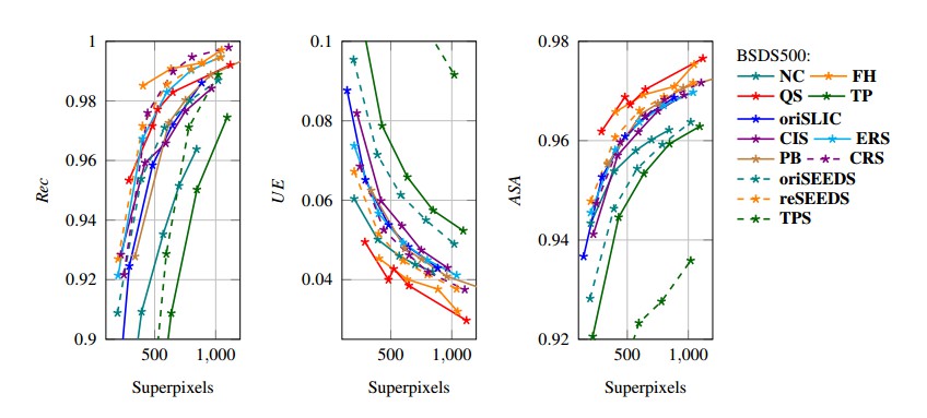
Superpixel algorithms are usually assessed using two measures: Boundary Recall and Undersegmentation Error. Let $S = \{S_1, \ldots, S_K\}$ be a superpixel segmentation and $G = \{G_1, ..., G_L\}$ be a ground truth segmentation. Then, Boundary Recall $Rec(S,G)$ is defined as follows:

$Rec(S,G) = \frac{TP(S, G)}{TP(S, G) + FN(S, G)}$

where $TP(S,G)$ is the number of boundary pixels in $G$ for which there is a boundary pixel in $S$ in range $r$ and $FN(S, G)$ is the number of boundary pixels in $G$ for which there is no boundary pixel in $S$ in range $r$. The range $r$ is set to $0.0075$ times the image diagonal and represents a tolerance parameter. Intuitively, Boundary Recall is the fraction of boundary pixels in $G$ which are correctly detected in $S$. The higher Boundary Recall, the better the superpixels adhere to object boundaries.

Undersegmentation Error measures the "leakage" of superpixels with respect to the ground truth segmentation. Formally, Undersegmentation Error $UE(S, G)$ is defined as

$UE(S,G) = \frac{1}{N} \sum_{G_i \in G} \sum_{S_j \cap G_i \neq \emptyset} \min \{|S_j \cap G_i|, |S_j - G_i|\}$

where $N$ is the number of pixels and $S_j - G_i = \{x \in S_j | x \notin G_i\}$. The lower the Undersegmentation Error, the better the superpixels match the ground truth segments.

Achievable Segmentation Acurracy labels superpixels according to their underlying ground truth segments and counts the correctly labeled pixels [11]:

$ASA(S, G) = \frac{1}{N} \sum_{S_j \in S} \max_{G_i} \{|S_j \cap G_i|\}.$

This means, that Achievable Segmentation Accuracy represents an upper bound on the accuracy achievable by a subsequent segmentation step

Comparison

A thorough comparison of these superpixel algorithms can be found in my bachelor thesis: Bachelor Thesis “Superpixel Segmentation Using Depth Information”

The parameters of all algorithms were optimized on the validation set of the Berkeley Segmentation Dataset. The comparison in figure 1 is based on the test set. Note that not all superpixels ensure that the requested number of superpixels is met exactly. In figure 1, reSEEDS is the implementation of SEEDS used for my bachelor thesis, Bachelor Thesis “Superpixel Segmentation Using Depth Information”, and oriSEEDS is the original implementation. oriSLIC refers to the original implementation of SLIC.

reSEEDS, the implementation of SEEDS as part of my bachelor thesis is available on GitHub: SEEDS Revised on GitHub.

References

• [1] X. Ren, J. Malik. Learning a classification model for segmentation. International Conference on Computer Vision, pages 10–17, 2003.
• [2] J. Shi, J. Malik. Normalized cuts and image segmentation. Transactions on Pattern Analysis and Machine Intelligence, 22(8):888–905, 2000.
• [3] P. F. Felzenswalb, D. P. Huttenlocher. Efficient graph-based image segmentation. International Journal of Computer Vision, 59(2), 2004.
• [4] A. Vedaldi, S. Soatto. Quick shift and kernel methods for mode seeking. European Conference on Computer Vision, pages 705–718, 2008.
• [5] A. Levinshtein, A. Stere, K. N. Kutulakos, D. J. Fleet, S. J. Dickinson, K. Siddiqi. TurboPixels: Fast superpixels using geometric flows. Transactions on Pattern Analysis and Machine Intelligence, 31(12):2290–2297, 2009.
• [6] C. Rohkohl, K. Engel. Efficient image segmentation using pairwise pixel similarities. Pattern Recognition, volume 4713 of Lecture Notes in Computer Science, pages 254–263, 2007.
• [7] R. Achanta, A. Shaji, K. Smith, A. Lucchi, P. Fua, S. Süsstrunk. SLIC superpixels. Technical report, École Polytechnique Fédérale de Lausanne, 2010.
• [8] M. van den Bergh, X. Boix, G. Roig, B. de Capitani, L. van Gool. SEEDS: Superpixels extracted via energy-driven sampling. European Conference on Computer Vision, pages 13–26, 2012.
• [9] C. Conrad, M. Mertz, R. Mester. Contour-relaxed superpixels. Energy Minimization Methods in Computer Vision and Pattern Recognition, volume 8081 of Lecture Notes in Computer Science, pages 280–293, 2013.
• [10] O. Veksler, Y. Boykov, P. Mehrani. Superpixels and supervoxels in an energy optimization framework. European Conference on Computer Vision, pages 211–224, 2010.
• [11] M. Y. Lui, O. Tuzel, S. Ramalingam, R. Chellappa. Entropy rate superpixel segmentation. Conference on Computer Vision and Pattern Recognition, pages 2097–2104, 2011.
• [12] Y. Zhang, R. Hartley, J. Mashford, S. Burn. Superpixels via pseudo-boolean optimization. International Conference on Computer Vision, pages 1387–1394, 2011.
• [13] D. Tang, H. Fu, X. Cao. Topology preserved regular superpixel. International Conference on Multimedia and Expo, pages 765–768, 2012.