This paper proposes a graph based image segmentation technique which can be applied to a given superpixel segmentation, as well. An image is interpreted as weighted undirected graph $G = (V,E)$. If a superpixel segmentation is given, each superpixel forms a node, otherwise each pixel represents a node. The goal is to bipartition the graph into two disjoint sets $A \subset V$ and $B \subset V$ by minimizing the normalized cut $NCut(A, B)$ given by

$NCut(A, B) = \frac{cut(A, B)}{assoc(A, V)} + \frac{cut(A, B)}{assoc(A, V)}$.

Here, $cut(A, B) = \sum_{u \in A, v \in B} w_{u,v}$ and $assoc(A ,V) = \sum_{u \in A, v \in V} w_{u,v}$ where $w_{u,v}$ denotes the weight between node $u$ and node $v$ (we assume a fully connected graph where $w_{u,v}$ may be zero).

As shown in the paper, this criterion can be minimized by discretizing the second smallest eigenvalue corresponding to the generalized eigenvalue problem

$(D - W)y = \lambda D y$.

Assuming the nodes to be consecutively numbered, the matrix $W$ holds the edge weights: $W_{u, v} = w_{u,v}$, and thus is symmetric. $D$ is a diagonal matrix where $D_{u,u} = \sum_{v \in V} w_{u,v}$. The edge weights $w_{u,v}$ can for example be defined as follows: $w_{u,v} = \exp(\| I(u) - I(v) \|_2^2/\sigma^2)$ if superpixels $u$ and $v$ have a common border, $w_{u,v} = 0$ otherwise. In this case, $I(u)$ denotes the color vector of the superpixel corresponding to node $u$ (this may be the mean color of the superpixel). The second smallest eigenvector needs to be discretized. Therefore, Shi et al. choose a threshold value minimizing the normalized cut. Further details can be found in the paper. Code is available online: original MatLab code and an implementation by Gori to generate superpixels.

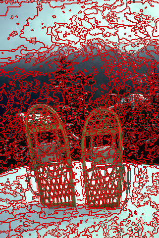
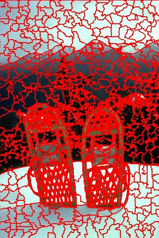
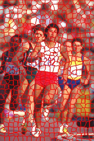
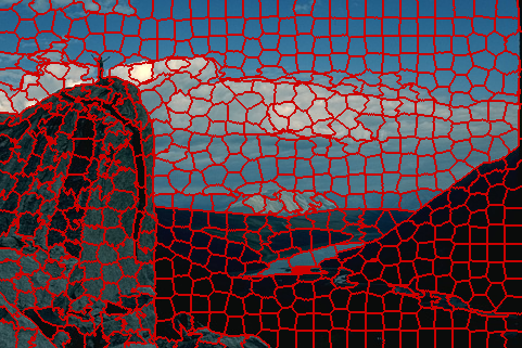
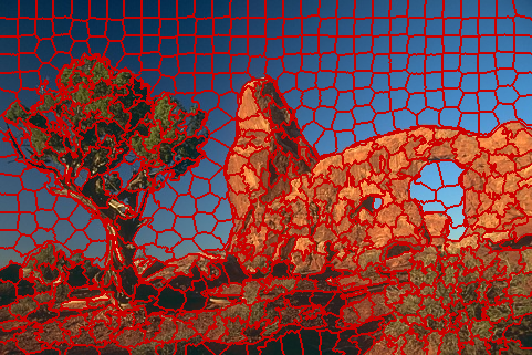
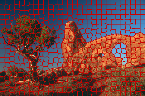
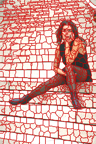
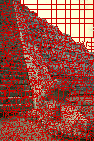
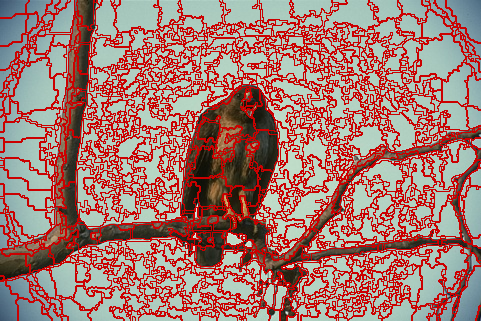
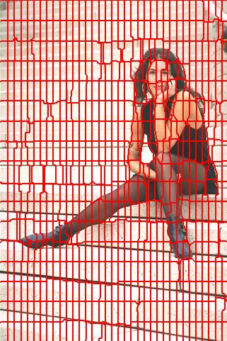
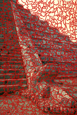
After introducing SEEDS [1] and SLIC [2], this article focusses on another approach to superpixel segmentation proposed by Felzenswalb & Huttenlocher. The procedure is summarized in algorithm 1 and based on the following definitions. Given an image $I$, $G = (V, E)$ is the graph with nodes corresponding to pixels, and edges between adjacent pixels. Each edge $(n,m) \in E$ is assigned a weight $w_{n,m} = \|I(n) - I(m)\|_2$. Then, for subsets $A,B \subseteq V$ we define $MST(A)$ to be the minimum spanning tree of $A$ and

$Int(A) = max_{n,m \in MST(A)} \{w_{n,m}\}$,

$MInt(A,B) = min\{Int(A) + \frac{\tau}{|A|}, Int(B) + \frac{\tau}{|B|}\}$.

where $\tau$ is a threshold parameter and $MInt(A,B)$ is called the minimum internal difference between components $A$ and $B$. Starting from an initial superpixel segmentation where each pixel forms its own superpixel the algorithm processes all edges in order of increasing edge weight. Whenever an edge connects two different superpixels, these are merged if the edge weight is small compared to the minimum internal difference.

function fh(
        $G = (V,E)$ // Undirected, weighted graph.
    )
    sort $E$ by increasing edge weight
    let $S$ be the initial superpixel segmentation
    for $k = 1,\ldots,|E|$
        let $(n,m)$ be the $k^{\text{th}}$ edge
            if the edge connects different superpixels $S_i,S_j \in S$
                if $w_{n,m}$ is sufficiently small compared to $MInt(S_i,S_j)$
                    merge superpixels $S_i$ and $S_j$
    return $S$

The original implementation can be found on Felzenswalb's website. Generated superpixel segmentations can be found in figure 1.

• [1] R. Achanta, A. Shaji, K. Smith, A. Lucchi, P. Fua, S. Süsstrunk. SLIC superpixels. Technical report, École Polytechnique Fédérale de Lausanne, 2010.
• [2] M. van den Bergh, X. Boix, G. Roig, B. de Capitani, L. van Gool. SEEDS: Superpixels extracted via energy-driven sampling. European Conference on Computer Vision, pages 13–26, 2012.
• [3] P. Arbeláez, M. Maire, C. Fowlkes, J. Malik. Contour detection and hierarchical image segmentation. Transactions on Pattern Analysis and Machine Intelligence, volume 33, number 5, pages 898–916, 2011.

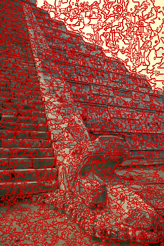
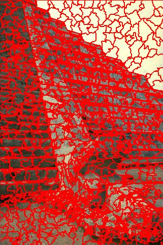
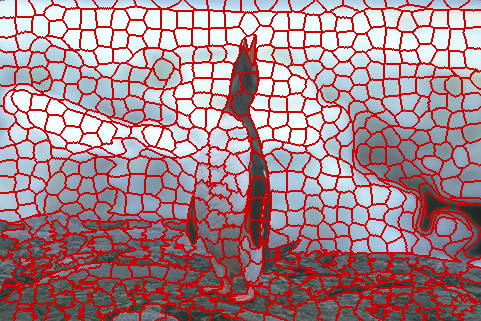
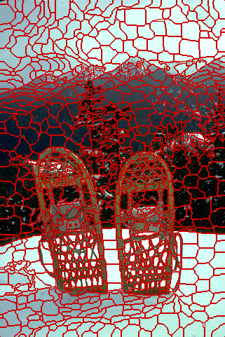
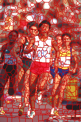
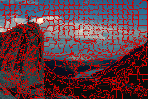
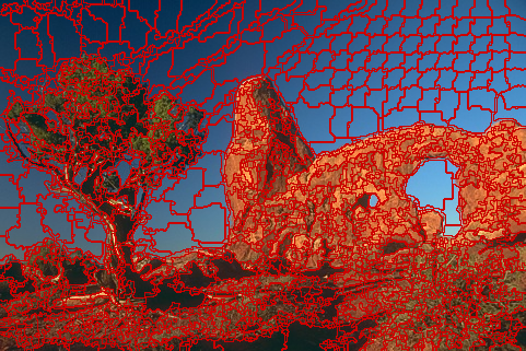
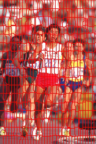
Proposed in 2008, Quick Shift is a segmentation algorithm based on mode seeking which can also be used to generate superpixels. In general, a mode seeking algorithm starts from a Parzen density estimate $p(x_n)$ for all pixels $x_n \in \{1,\ldots,W\} \times \{1,\ldots,H\}$ (here, $W$ and $H$ are the width and height of the image, respectively) and each pixel is assigned to a mode by following the density $p(x_n)$ upwards, that is in the direction of the gradient. Therefore, Quick Shift may be categorized as gradient ascent method. In particular, Quick Shift pre-computes $p(x_n)$ for all pixels using a Gaussian kernel. In practice, given an image $I$, the distance $d(x_n, x_m)$ used within the Gaussian kernel consists of a color term and a spatial term:

$d(x_n, x_m) = α \| I(x_n)−I(x_m)\|_2 + \|x_n −x_m\|_2$

where $α$ weights the influence of the color term. Subsequently, each pixel $x_n$ gets assigned to the pixel $x_m \in N_R(x_n) = \{x_m : \|x_n −x_m\|_\infty \leq R/2\}$ such that $p(x_m) > p(x_n)$ or is left unassigned. These assignments correspond to the modes, which represent the final superpixels. The algorithm is summarized in algorithm 1.

function quickshift(
        $I$ // Color image.
    )
    for $n = 1$ to $W\cdot H$
        initialize $t(x_n) = 0$
    for $n = 1$ to $W\cdot H$
        // $N_R(x_n)$ is the set of all pixels in the neighborhood of size $N$ around $x_n$.
        calculate $p(x_n) = \sum_{x_m \in N_R(x_n)} \exp\left(\frac{-d(x_n, x_m)}{(2/3)R}\right)$
    for $n = 1$ to $W\cdot H$
        set $t(x_n) = \arg \max_{x_m \in N_R(x_n):p(x_m) > p(x_n)}\{p(x_m)\}$
    // $t$ can be interpreted as forest, where all pixels $x_n$ with $t(x_n) = 0$ are roots.
    derive superpixel segmentation $S$ from $t$
    return $S$

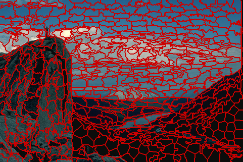
The original implementation is part of the VLFeat Library. Generated superpixel segmentations can be found in figure 1.

• [1] P. Arbeláez, M. Maire, C. Fowlkes, J. Malik. Contour detection and hierarchical image segmentation. Transactions on Pattern Analysis and Machine Intelligence, volume 33, number 5, pages 898–916, 2011.

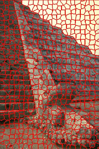
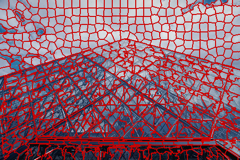
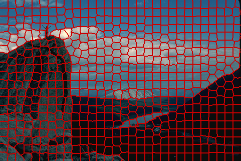
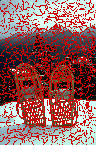
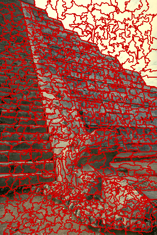
TurboPixels is one of the first superpixel algorithms (that is, the algorithm was, in contrast to Quick Shift [1] and the approach by Felzenswalb and Huttenlocher [2], originally intended to generate superpixels). Inspired by active contours, after placing superpixel centers on a reglar grid, the superpixels are grown based on an evolving contour. The contour is implemented as level set of the function

$\psi : \mathbb{R}^2 \times [0, \tau) \rightarrow \mathbb{R}^2$.

The evolution is formally defined by

$\psi_t = -v \|\ \nabla \psi\|_2$

where $\nabla\psi$ denotes the gradient of $\psi$ and $\psi_t$ is the temporal derivative. Here, the speed $v$ describes the future evolution of the contour. In practive, $\psi$ will be the signed euclidean distance and evolution is carried out using a first-order discretization. The contour in iteration $(T + 1)$ is given by

$\psi^{(T+1)} = \psi^{(T)} - v_I v_B \|\nabla \psi^{(T)}\|\Delta t$.

The speed $v$ is split up into two components: $v_I$ which depends on the image content and $v_B$ which ensures that superpixels do not overlap. Iteratively, the superpixels are grown by computing $v_I$ and $v_B$ and then applying the equation above, see the paper for details. The procedure is summarized in algorithm 1.

function turbopixels(
        $I$, // Color image.
        $K$, // Number of superpixels.
    )
    place initial superpixel centers on a regular grid
    initialize $\psi^{(0)}$
    repeat
        compute $v_I$ and $v_B$
        evolve the contour by computing $\psi^{(T+1)}$
        update assigned pixels
        $T := T + 1$
    until all pixels are assigned
    derive superpixel segmentation $S$ from $\psi$
    return $S$

The original MatLab implementation is available online on Alex Levinshten's homepage. Figure 1 shows superpixel segmentations generated by TurboPixels.

• [1] A. Vedaldi, S. Soatto. Quick Shift and Kernel Methods for Mode Seeking. European Conference on Computer Vision, 2008.
• [2] P. F. Felzenswalb and D. P. Huttenlocher. Efficient graph-based image segmentation. International Journal of Computer Vision, volume 59, number 2, 2004.
• [3] P. Arbeláez, M. Maire, C. Fowlkes, J. Malik. Contour detection and hierarchical image segmentation. Transactions on Pattern Analysis and Machine Intelligence, volume 33, number 5, pages 898–916, 2011.

Achanta et al. proposed their superpixel algorithm "Simple Linear Iterative Clustering", short SLIC, in [1]. The above paper compares SLIC to several superpixel algorithms with respect to Boundary Recall, Undersegmentation Error and runtime: Normalized Cuts [2], the approach proposed by Felzenswalb and Huttenlocher [3], Quick Shift [4], Watersheds [5] and Turbopixels [6].

Update. Thorough evaluation of both implementations can be found in my bachelor thesis: Bachelor Thesis “Superpixel Segmentation Using Depth Information”.

Figure 1: Superpixel segmentations with roughly $600$ superpixels generated by the original implementation of SLIC which allows to adjust the compactness of the superpixels. The images are taken from the validation set of the Berkeley Segmentation Dataset [8]. From top to bottom: compactness set to $1$; compactness set to $10$; compactness set to $40$.

• [1] R. Achanta, A. Shaji, K. Smith, A. Lucchi, P. Fua, S. Susstrunk. SLIC Superpixels. Technical report, EPFL, Lausanne, 2010.
• [2] X. Ren, J. Malik. Learning a classification model for segmentation. Proceedings of the International Conference on Computer Vision, pages 10–17, 2003.
• [3] P. F. Felzenswalb, D. P. Huttenlocher. Efficient graph-based image segmentation. International Journal of Computer Vision, volume 59, number 2, 2004.
• [4] A. Vedaldi, S. Soatto. Quick shift and kernel methods for mode seeking. Proceedings of the European Conference on Computer Vision, pages 705–718, 2008.
• [5] L. Vincent, P. Soille. Watersheds in digital spaces: An efficient algorithm based on immersion simulations, Transactions on Pattern Analysis and Machine Intelligence, volume 13, number 6, pages 583-598, 1991.
• [6] A. Levinshtein, A. Stere, K. N. Kutulakos, D. J. Fleet, S. J. Dickinson, K. Siddiqi. TurboPixels: Fast superpixels using geometric flows. Transactions on Pattern Analysis and Machine Intelligence, volume 31, number 12, pages 2290–2297, 2009.
• [7] A. Vedaldi, B. Fulkerson. VLFeat: An open and portable library of computer vision algorithms. http://www.vlfeat.org/, 2008.
• [8] P. Arbeláez, M. Maire, C. Fowlkes, J. Malik. Contour detection and hierarchical image segmentation. Transactions on Pattern Analysis and Machine Intelligence, volume 33, number 5, pages 898–916, 2011.

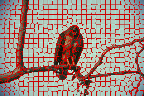
Veksler et al. propose a graph based superpixel algorithm - to be exact, the paper proposes two algorithms: Compact Superpixels and Constant Intensity Superpixels. In the following we focus on Constant Intensity Superpixels, as the algorithm shows better performance in practice. Note that we assume the image $I$ to be a grayscale image, however, the below description can easily be extended to color images. Initially the image is covered by overlapping squares such that each pixel is covered by multiple squares. Each square represents a superpixel and each pixel can get assigned to one of these squares. Then, the following energy is minimized using $\alpha$-expansion [1]:

$E(S) = \sum _{n = 1}^N\sum_{m = 1}^N w_{n,m} \psi_{n,m}(s(x_n), s(x_m)) + \sum_{n = 1}^N \theta_n(s(x_n))$

where $N$ is the number of pixels and $s(x_n)$ denotes the label of pixel $x_n$. Here, $\theta_n$ defines a data term which can be written as

$\theta_n(i) = |I(x_n) - I(S_i)|$, if $x_n$ is assigned to superpixel $S_i$, $0$ otherwise.

Note that this is a simplified formulation: Originally, instead of using the mean color $I(S_i)$ of the superpixel $S_i$, the color of the center pixel of the initial square is used (however, this would require to discuss an additional term enforcing this pixel to belong to $S_i$). Further, $\psi_{n,m}$ is a Potts model:

$\psi_{n,m}(i, j) = 1$, if $i \neq j$, $0$ otherwise.

The weights $w_{n,m}$ of neighboring pixels $x_n$ and $x_m$ are defined as follows:

$w_{n,m} = \lambda \exp\left(- \frac{(I(x_n) - I(x_m))^2}{2 \|x_n - x_m\|_2 \sigma^2}\right)$

where $\lambda$ is an adjustable parameter and $\sigma$ is set to the overall variance of the image.

Figure 1 shows superpixel segmentations obtained for images of the Berkeley Segmentation Dataset [2] using the original implementation available on Olga Veksler's webpage.

• [1] Y. Boykov, O. Veksler, R. Zabih. Fast approximate energy minimization via graph cuts. Transactions on Pattern Analysis and Machine Intelligence, Transactions on, pages 1222–1239, 2001.
• [2] P. Arbeláez, M. Maire, C. Fowlkes, J. Malik. Contour detection and hierarchical image segmentation. Transactions on Pattern Analysis and Machine Intelligence, volume 33, number 5, pages 898–916, 2011.

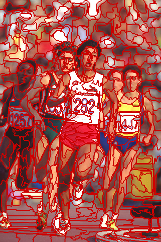
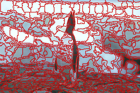
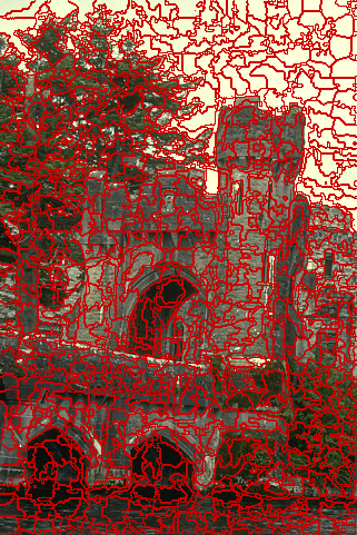
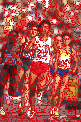
Another graph-based method for superpixel segmentation was proposed by Lui et al. Using greedy optimization, summarized in algorithm 1, an objective function based on the entropy rate of a random walk on the graph $\hat{G} = (V,M)$ with $M \subseteq E$ is proposed (where we interpret the image $I$ as 4-connected graph $G = (V,E)$):

$E(\hat{G}) = H(\hat{G}) + \lambda B(\hat{G})$

where $H(\hat{G})$ refers to the entropy rate of the randon walk, while $B(\hat{G})$ defines a balancing term. The objective is maximized subject to the constraint that the number of connected components in $\hat{G}$ is equal or lower to the desired number of superpixels $K$. Given weights $w_{n,m}$ between pixels $x_n$ and $x_m$, defined using a Gaussian kernel based on the $L_1$ color distance, $H(\hat{G})$ is defined as:

$H(\hat{G}) = - \sum_{n = 1}^N \frac{w_n}{\sum_{m = 1}^N w_m} \sum_{m = 1}^N p_{n,m} \log(p_{n,m})$

where we set $w_n = \sum_{m = 1}^N w_{n,m}$ and $N$ denotes the number of pixels. Here, the probabilities $p_{n,m}$ refer to the transition probabilities of the random walk and can be calculated as

$p_{n,m} = \frac{w_{n,m}}{w_n}$ if $n \neq m$ and $(n,m) \in M$,
$p_{n,m} = 1 - \frac{\sum_{m = 1:(n,m) \in M}^N w_{n,m}}{w_n}$ if $n \neq m$ and $(n,m) \notin M$,
$p_{n,m} = 0$ otherwise.

The balacing term favors superpixels of approximately the same size (regarding the number of pixels):

$B(\hat{G}) = - \sum_{i = 1}^K \frac{|S_i|}{N} log\left(\frac{|S_i|}{N}\right)$.

where $S_i$ denotes the $i^\text{th}$ superpixel. Starting from an initial superpixels segmentation where each pixel forms its own superpixel, the algorithm greedily adds edges to merge superpixels until the desired number of superpixels is reached, see algorithm 1.

function ers(
        $G = (V,E)$ // Undirected weighted graph.
    )
    initialize $M = \emptyset$
    for each edge $(n,m) \in E$
        // Let $\hat{G}$ denote the graph $(V, M \cup \{(n,m)\})$:
        let $(n,m)$ be the edge yielding the largest gain in the energy $E(\hat{G})$
        if $\hat{G}$ contains $K$ connected components or less:
            $M := M \cup \{(n,m)\}$.
    derive superpixel segmentation $S$ from $\hat{G}$
    return $S$

The implementation is availabel online at mingyuliu.net. Figure 1 shows several images from the Berkeley Segmentation Dataset [1] oversegmented using the approach described above.

• [1] P. Arbeláez, M. Maire, C. Fowlkes, J. Malik. Contour detection and hierarchical image segmentation. Transactions on Pattern Analysis and Machine Intelligence, volume 33, number 5, pages 898–916, 2011.

Zhang et al. propose a graph-based superpixel algorithm. First, the image is covered by overlapping vertical and horizontal strips such that each pixel is covered by exactly two vertical and two horizontal strips. This way, considering only the horizontal strips, each pixel is either labeled 0 or 1. $N$ being the number of nodes (that is, pixels), an energy similar to the one used for Constant Intensity Superpixels [1] is used:

$E(S) = \sum _{n = 1}^N\sum_{m = 1}^N w_{n,m} \psi_{n,m}(s(x_n), s(x_m)) + \sum_{n = 1}^N \theta_n(s(x_n))$

except that the data term $\theta_n$ is set to zero. The smoothing term $\psi_{n,m}$ is based on the following consideration. Numbering the horizontal strips such that $H_i \subseteq V$ is covered halfway by $H_{i + 1} \subseteq V$, where $V$ is the set of all nodes (that is, pixels), and considering neighboring pixels $x_n$ and $x_m$ such that $x_n$ lies above or at the same horizontal line as $x_m$, three cases are possible:

$x_n \in H_i \cap H_{i + 1}$ and $x_m \in H_i \cap H_{i + 1}$,
$x_n \in H_i \cap H_{i + 1}$ and $x_m \in H_{i+1} \cap H_{i+2}$,
$x_n \in H_i \cap H_{i+1}$ and $x_m \in H_{i+1} \cap H_{i+2}$,

Including two possible labels per pixel, there are twelve cases to consider. These cases get assigned different weights $w_{n,m}$ which are computed using a Gaussian kernel and the $L_1$ color distance, see their paper. The energy is optimized using max-flow. The final superpixel segmentation can be derived from the vertical and horizontal labels.

A C++ implementation is available at Zhang's webpage. Figure 1 shows superpixel segmentations obtained using the algorithm described above.

• [1] O. Veksler, Y. Boykov, P. Mehrani. Superpixels and supervoxels in an energy optimization framework. European Conference on Computer Vision, pages 211–224, 2010.
• [2] P. Arbeláez, M. Maire, C. Fowlkes, J. Malik. Contour detection and hierarchical image segmentation. Transactions on Pattern Analysis and Machine Intelligence, volume 33, number 5, pages 898–916, 2011.

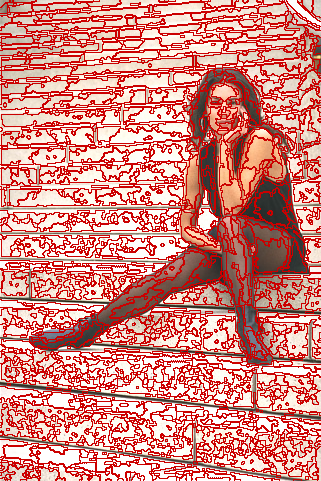
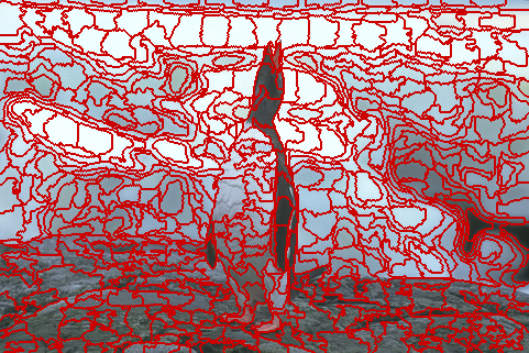
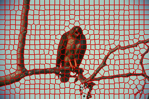
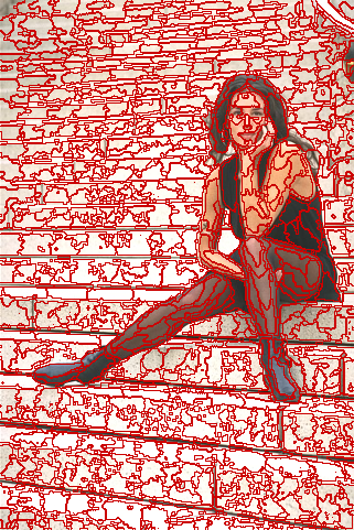
Van den Bergh et al. propose a superpixel algorithm called SEEDS using color histograms to refine an initial superpixel segmentation. The main goal of my bachelor thesis is the integration of depth information into SEEDS, see my bachelor thesis proposal and the slides of my introductory talk. Figure 1 shows images from the validation set of the Berkeley Segmentation Dataset [1] oversegmented using the original implementation of SEEDS.

Update. Thorough evaluation of both the original implementation and my implementation of SEEDS can be found in my bachelor thesis: Bachelor Thesis “Superpixel Segmentation Using Depth Information”.

• [1] P. Arbeláez, M. Maire, C. Fowlkes, J. Malik. Contour detection and hierarchical image segmentation. Transactions on Pattern Analysis and Machine Intelligence, volume 33, number 5, pages 898–916, 2011.

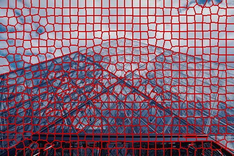
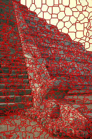
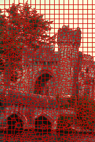
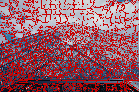
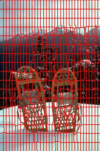
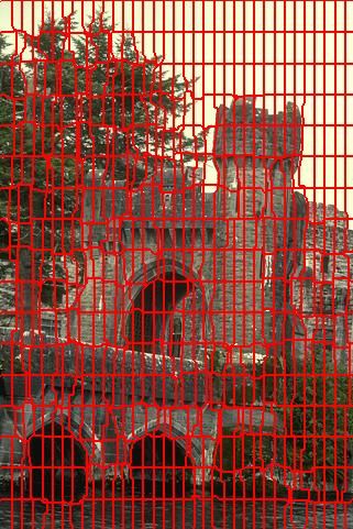
Tang et al. propose a superpixel algorithm which generates a regular grid of superpixels, that is the superpixels can be arranged in an array where each superpixel has a consistent, ordered position. Given an edge map

$p: \{1,\ldots,W\} \times \{1,\ldots,H\} \rightarrow [0,1], x_n \mapsto p(x_n)$

defining the probability of an edge being present at pixel $x_n$, the algorithm proceeds in three steps. Firstly, a set of pixels are chosen as initial grid positions. This is done on a regular grid with horizontal step size $R_h$ and vertical step size $R_v$ given as

$R_v \approx \sqrt{\frac{K H}{W}}$, $R_h = \frac{K}{R_v}$

where $K$ is the desired number of superpixels. Let $\mu_1,\ldots,\mu_{K'}$ denote these positions (where $K'$ is the number of grid positions required to obtain $K$ superpixels). Secondly, the positions are moved towards maximum edge positions by choosing

$\mu_i = arg \max_{x_n \in N_R(\mu_i)}\{p(x_n) \exp(\frac{\|x_n − \mu_i\|_2}{2 \sigma})\}$

where $N_R(\mu_i)$ defines a local search region around the position $\mu_i$. Finally, these grid positions define an undirected graph based on their relative positions. Neighboring positions are connected by the shortest path calculated on the undirected, weighted graph with weights

$w_{n,m} = \frac{1}{p(x_n) + p(x_m)}$

for neighboring pixels $x_n$ and $x_m$. The shortest path is computed using Dijkstra’s algorithm. The superpixels are then given by the enclosed regions.

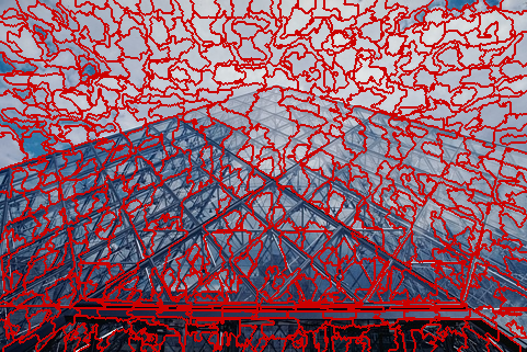
An implementation is available on Fu's webpage. Figure 1 shows superpixels segmentations obtained using Topology Preserving Superpixels.

• [1] P. Arbeláez, M. Maire, C. Fowlkes, J. Malik. Contour detection and hierarchical image segmentation. Transactions on Pattern Analysis and Machine Intelligence, volume 33, number 5, pages 898–916, 2011.

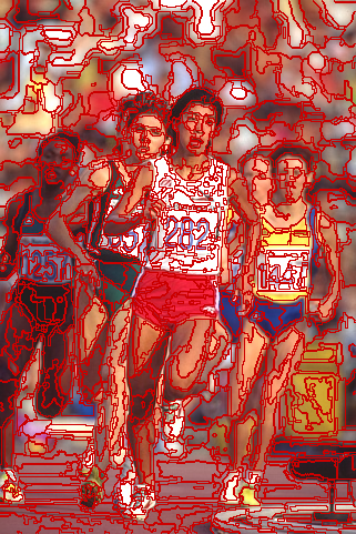
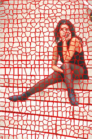
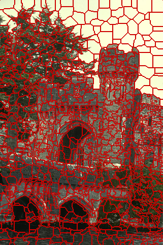
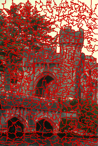
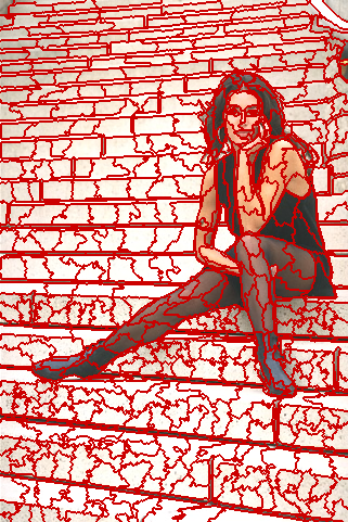
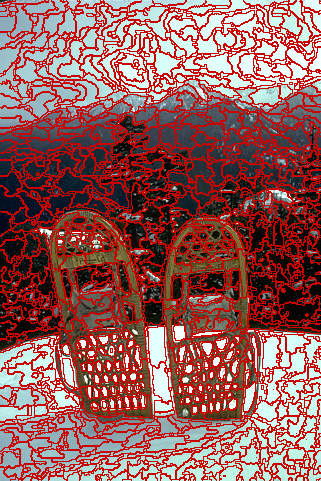
This paper introduces Contour Relaxed Superpixels, a statistical approach to superpixel segmentation. In particular, the value $I_c(x_n)$ of pixel $x_n$ in channel $c$ is assumed to be the outcome of stochastic process described by the parameters $\theta_{s(x_n), c}$ of the corresponding superpixel $S_{s(x_n)}$ where $s(x_n)$ denotes the superpixel $x_n$ belongs to. Using $\theta$ to denote the set of all such parameters, the superpixel segmentation $S$ maximizing $p(S, \theta | I)$ is searched for. Using bayes theorem, and omitting the normalization factor, the energy to be maximized is given by

$p(S, \theta | I) = \frac{p(I | S, \theta) p(S, \theta)}{p(I)} \propto p(I |S, \theta) p(S, \theta) =: E(S)$.

The parameters $\theta$ are considered deterministic parameters such that $p(S, \theta)$ can be simplified to $p(S, \theta) = \kappa p(S)$. An EM-style (e.g. see [1, p. 423ff]) algorithm is applied: The parameters $\theta$ are optimized using maximum likelihood considering the superpixel segmentation to be constant followed by optimizing for $S$ while the parameters $\theta$ are held constant. Considering each pixel connected to $8$ neighbors, $p(S)$ is modeled using a Gibbs Random Field and can be factorzed into

$p(S) = \kappa' \exp(-N_e C_e - N_v C_v)$

where only the second factor depends on the label of the pixel $x_n$. Here, $N_e$ is the number of direct neighbors of $x_n$ having a different label and $N_v$ is the number of diagonal neighbors with a different label ‐ $C_e$ and $C_v$ are the associated costs. Furtermore, the probability $p(I | S, \theta)$ can be factorized as

$p(I | S, \theta) = \prod _{S_i \in S}\prod_{x_n \in S_i} \prod_{c=1}^3 p(I_c(x_n) | \theta_{i,c})$

where all the stoachstic processes are considered independent.

The optimization is carried out as follows: Iteratively, each boundary pixel $x_n$ is considered to change its label. When $\theta$ is assumed constant, $x_n$ is assigned the label maximizing

$E(S) = \kappa \kappa' \exp(-N_e C_e - N_v C_v) \prod_{S_i} \prod_{x_m \in S_i}\prod_{c=1}^3 p(I_c(x_m)|\theta_{i,c})$.(1)

This approach can be categorized as gradient ascent approach to superpixel segmentation and is summarized in algorithm 1. The first product in equation (1) runs over all superpixels $S_i$ to which pixel $x_n$ may be assigned.

function crs(
        $I$, // Color image.
        $K$ // Number of superpixels.
    )
    // The step size R can be derived from the image size W ×H and K:
    initialize $S$ as regular grid with step size $R$
    initialize $\theta$ using sufficient statistics (e.g. Gaussian)
    for $t = 1$ to $T$
        // Originally, the image is traversed multiple times using different
        // directions to avoid a directional bias:
        for $n = 1$ to $N$
            if $x_n$ is a boundary pixel
                // This can be evaluated by taking θ as constant; Conrad et al.
                // suggest to minimize the negative logarithm of (1) instead:
                assign $x_n$ to the label maximizing equation (1)
    return $S$

A C++ implementation of Contour Relaxed Superpixels is available at the project's webpage. Superpixel segmentations generated using the described approach are shown in figure 1.

• [1] C. Bishop. Pattern Recognition and Machine Learning. Springer Verlag, New York, 2006.
• [2] P. Arbeláez, M. Maire, C. Fowlkes, J. Malik. Contour detection and hierarchical image segmentation. Transactions on Pattern Analysis and Machine Intelligence, volume 33, number 5, pages 898–916, 2011.