Recognizing Handwritten Digits using a Two-Layer Perceptron and the MNIST Dataset

Foreword

In the course of a seminar on “Selected Topics in Human Language Technology and Pattern Recognition” I wrote a seminar paper on neural networks: "Introduction to Neural Networks". The seminar paper and the slides of the corresponding talk can be found in my previous article: Seminar Paper “Introduction to Neural Networks”. Background on neural networks and the two-layer perceptron can be found in my seminar paper.

Introduction

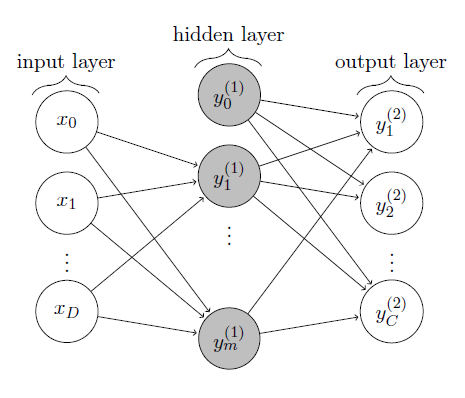
The MNIST dataset provides a training set of $60,000$ handwritten digits and a validation set of $10,000$ handwritten digits. The images have a size of $28 \times 28$ pixels. We want to train a two-layer perceptron to recognize handwritten digits, that is given a new $28 \times 28$ pixels image, the goal is to decide which digit it represents. For this purpose, the two-layer perceptron consists of $28 \cdot 28 = 784$ input units, a variable number of hidden units and $10$ output units. The general case of a two-layer perceptron with $D$ input units, $m$ hidden units and $C$ output units is shown in figure 1.

Figure 1: A two-layer perceptron with $D$ input units, $m$ hidden units and $C$ output units.

Code

The two-layer perceptron is implemented in MatLab and the code can be found on GitHub and is available under the GNU General Public License version 3.

The methods loadMNISTImages and loadMNISTLabels are used to load the MNIST dataset as it is stored in a special file format. The methods can be found online at http://ufldl.stanford.edu/wiki/index.php/Using_the_MNIST_Dataset.

Code on GitHub

Network Training

The network is trained using a stochastic variant of mini-batch training, the sum-of-squared error function and the error backpropagation algorithm. The method returns the weights of the hidden layer and the output layer after training as well as the normalized sum-of-squared error after the last iteration. In addition, it plots the normalized error over time resulting in a plot as shown in figure 2.

function [hiddenWeights, outputWeights, error] = trainStochasticSquaredErrorTwoLayerPerceptron(activationFunction, dActivationFunction, numberOfHiddenUnits, inputValues, targetValues, epochs, batchSize, learningRate)
% trainStochasticSquaredErrorTwoLayerPerceptron Creates a two-layer perceptron
% and trains it on the MNIST dataset.
%
% INPUT:
% activationFunction             : Activation function used in both layers.
% dActivationFunction            : Derivative of the activation
% function used in both layers.
% numberOfHiddenUnits            : Number of hidden units.
% inputValues                    : Input values for training (784 x 60000)
% targetValues                   : Target values for training (1 x 60000)
% epochs                         : Number of epochs to train.
% batchSize                      : Plot error after batchSize images.
% learningRate                   : Learning rate to apply.
%
% OUTPUT:
% hiddenWeights                  : Weights of the hidden layer.
% outputWeights                  : Weights of the output layer.
%

Figure 2: The normalized error plotted during training with a learning rate $\gamma = 0.5$, $500$ hidden units, a batch size of $100$ images iterated $500$ times. The $y$-axis represents the normalized error; the $x$-axis is the iteration.

The above method requires the activation function used for both the hidden layer and the output layer to be given as parameter. The logistic sigmoid defined by

$\sigma(z) = \frac{1}{1 + \exp(-z)}$

is a commonly used activation function and implemented in logisticSigmoid. In addition, the error backpropagation algorithm needs the derivative of the activation function which is implemented as dLogisticSigmoid.

function y = logisticSigmoid(x)
% simpleLogisticSigmoid Logistic sigmoid activation function
% 
% INPUT:
% x     : Input vector.
%
% OUTPUT:
% y     : Output vector where the logistic sigmoid was applied element by
% element.
%

function y = dLogisticSigmoid(x)
% dLogisticSigmoid Derivative of the logistic sigmoid.
% 
% INPUT:
% x     : Input vector.
%
% OUTPUT:
% y     : Output vector where the derivative of the logistic sigmoid was
% applied element by element.
%

Usage and Validation

The method applyStochasticSquaredErrorTwoLayerPerceptronMNIST provides an example of how to use the above methods:

% Load MNIST dataset.
inputValues = loadMNISTImages('train-images.idx3-ubyte');
labels = loadMNISTLabels('train-labels.idx1-ubyte');
    
% Transform the labels to correct target values.
targetValues = 0.*ones(10, size(labels, 1));
for n = 1: size(labels, 1)
    targetValues(labels(n) + 1, n) = 1;
end;
    
% Choose form of MLP:
numberOfHiddenUnits = 700;
    
% Choose appropriate parameters.
learningRate = 0.1;
    
% Choose activation function.
activationFunction = @logisticSigmoid;
dActivationFunction = @dLogisticSigmoid;
    
% Choose batch size and epochs. Remember there are 60k input values.
batchSize = 100;
epochs = 500;
    
fprintf('Train twolayer perceptron with %d hidden units.\n', numberOfHiddenUnits);
fprintf('Learning rate: %d.\n', learningRate);
    
[hiddenWeights, outputWeights, error] = trainStochasticSquaredErrorTwoLayerPerceptron(activationFunction, dActivationFunction, numberOfHiddenUnits, inputValues, targetValues, epochs, batchSize, learningRate);
    
% Load validation set.
inputValues = loadMNISTImages('t10k-images.idx3-ubyte');
labels = loadMNISTLabels('t10k-labels.idx1-ubyte');
    
% Choose decision rule.
fprintf('Validation:\n');
    
[correctlyClassified, classificationErrors] = validateTwoLayerPerceptron(activationFunction, hiddenWeights, outputWeights, inputValues, labels);
    
fprintf('Classification errors: %d\n', classificationErrors);
fprintf('Correctly classified: %d\n', correctlyClassified);

First the MNIST dataset needs to be loaded using the methods mentioned above (loadMNISTImages and loadMNISTLaels). The labels are provided as vector where the $i^{th}$ entry contains the digit represented by the $i^{th}$ image. We transform the labels to form a $10 \times N$ matrix, where $N$ is the number of training images, such that the $i^{th}$ entry of the $n^{th}$ column vector is $1$ iff the $n^{th}$ training image represents the digit $i - 1$.

The network is trained using the logistic sigmoid activation function, a fixed batch size and a fixed number of iterations. The training method trainStochasticSquaredErrorTwoLayerPerceptron returns the weights of the hidden layer and the output layer as well as the normalized sum-of-squared error after the last iteration.

The method validateTwoLayerPerceptron uses the network weights to count the number of classification errors on the validation set.

Results

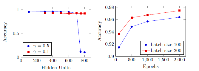
Some of the results after validating the two-layer perceptron on the provided validation set can be found in my seminar paper or in figure 3.

Figure 3: Results of the trained two-layer perceptron evaluated on the validation set of $10,000$ handwritten digits. Left: $500$ training iterations with a batch size of $100$ and the shown learning rates $\gamma = 0.5$ and $\gamma = 0.1$. Right: $500$ training iterations with fixed learning rate $\gamma = 0.5$ and batch sizes $100$ and $200$.

References

[1] David Stutz, Pavel Golik, Ralf Schlüter, and Hermann Ney. Introduction to Neural Networks. Seminar on Selected Topics in Human Language Technology and Pattern Recognition, 2014. PDF

IAM

DAVIDSTUTZ

ARTICLE