RESEARCH
Superpixel Benchmark (2016)
This page presents an extension to earlier research, see Superpixels Revisited. In particular, a comprehensive evaluation of 28 state-of-the-art algorithms on 5 different datasets is presented. To this end, a new benchmark was developed allowing to focus on a fair evaluation and designed to provide novel insights. The benchmark including all evaluated algorithms is available on GitHub. The corresponding paper is available on ArXiv.
Quick links: Paper | BibTex | Source Code | Submission
Overview
The main contribution of the work is a comprehensive and fair comparison of 28 superpixel algorithms. This is motivated by the growing number of algorithms as well as varying experimental setups, making direct comparison of reported results difficult. Therefore, parameter optimization is discussed explicitly and the importance of enforcing connectivity is discussed. Superpixel algorithms are evaluated based on qualitative and quantitative measures as well as runtime. Furthermore, the influence of noise and implementation details is investigated. Finally, commonly used metrics such as Boundary Recall [2] and Undersegmentation Error [3] are rendered independent of the number of superpixels allowing to provide a final ranking of superpixel algorithms.
The paper is available below, and the corresponding benchmark is available on GitHub:
Superpixel Benchmark on GitHubDownload and Citing
The paper can be downloaded below:
ArXiv Paper (∼ 4.3MB)
@article{StutzHermansLeibe:2016,
  author    = {David Stutz and Alexander Hermans and Bastian Leibe},
  title     = {Superpixels: An evaluation of the state-of-the-art},
  journal   = {Computer Vision and Image Understanding},
  volume    = {166},
  pages     = {1--27},
  year      = {2018},
  url       = {https://doi.org/10.1016/j.cviu.2017.03.007},
  doi       = {10.1016/j.cviu.2017.03.007},
}
Submission
In order to keep the presented benchmark alive, we encourage authors to submit their superpixel algorithms and the corresponding results. This also allows authors to compare their approaches to the state-of-the-art and report a reproducible and fair comparison in the corresponding publications.
Submission InstructionsNews & Updates
Apr 18, 2017. Interactive visualizations of qualitative and quanitative results have been added; fullscreen versions are also available: Qualitative Results, Quantitative Results. The source code can also be found on GitHub.
Apr 16, 2017. An implementation of the average metrics as described in the paper has been added to the benchmark. In addition, detailed instructions for adding/submitting new superpixel algorithms have been added to the documentation. The repository including documentaiton can be found here: davidstutz/superpixel-benchmark.
Apr 5, 2017. The reviews for the paper are summarized in this article: Reviews and Rebuttal for “Superpixels: An Evaluation of the State-of-the-Art”.
Mar 30, 2017. As of Mar 29, the paper was accepted for publication in Computer Vision and Image Understanding. The revised paper will be made available as soon as possible.
Feb 11, 2017. Thanks to Wanda Benesova, the source code of MSS has been added to the repository.
Jan 21, 2017. The NYUV2, SUNRGBD and SBD datasets are now available in the converted format used by the benchmark. Check out the data repository.
Jan 21, 2017. Thanks to John MacCormick and Johann Straßburg, the source code for PF and SEAW has been added to the repository.
Dec 20, 2016. Doxygen documentation (for the C++ parts, including the benchmark and several superpixel algorithms) is now available here.
Dec 11, 2016. As the presented paper was in preparation for a longer period of time, some recent superpixel algorithms are not included in the comparison — these include SCSP [38] and LRW [39]. To keep the benchmark up-to-date, these superpixel algorithms might be included in future updates.
Superpixel Algorithms
Table 1 gives a brief overview of the evaluated algorithms. Note that due to the high effort involved in running fair experiments and preparing them for publications, all publicly available superpixel algorithms up to (and including) 2015 are included. Additionally, some implementations that are not publicly available were provided by the corresponding authors. Unfortunately, many proposed algorithms were not evaluated due to missing implementations, see [1] for a list.
| Algorithm | Reference | Implementation | |
|---|---|---|---|
| W | [4], 1992 | C/C++ | Webpage |
| EAMS | [5], 2002 | MatLab/C | Webpage |
| NC | [6], 2003 | MatLab/C | Webpage |
| FH | [7], 2004 | C/C++ | Webpage |
| reFH | —"— | C/C++ | Webpage |
| RW | [8, 9], 2004 | MatLab/C | Webpage |
| QS | [10], 2008 | MatLab/C | Webpage |
| PF | [11], 2009 | Java | Webpage |
| TP | [12], 2009 | MatLab/C | Webpage |
| CIS | [13], 2010 | C/C++ | Webpage |
| SLIC | [14, 15], 2010 | C/C++ | Webpage |
| vlSLIC | —"— | C/C++ | Webpage |
| CRS | [16, 17], 2011 | C/C++ | Webpage |
| ERS | [18], 2011 | C/C++ | Webpage |
| PB | [19], 2011 | C/C++ | Webpage |
| DASP | [20], 2012 | C/C++ | Webpage |
| SEEDS | [21], 2012 | C/C++ | Webpage |
| reSEEDS | —"— | C/C++ | Webpage |
| TPS | [22, 23], 2012 | MatLab/C | Webpage |
| VC | [24], 2012 | C/C++ | Webpage |
| CCS | [25, 26], 2013 | C/C++ | Webpage |
| VCCS | [27], 2013 | C/C++ | Webpage |
| CW | [28], 2014 | C/C++ | Webpage |
| ERGC | [29, 30], 2014 | C/C++ | Webpage |
| MSS | [31], 2014 | C/C++ | — |
| preSLIC | [28], 2014 | C/C++ | Webpage |
| WP | [32, 33], 2014 | Python | Webpage |
| ETPS | [34], 2015 | C/C++ | Webpage |
| LSC | [35], 2015 | C/C++ | Webpage |
| POISE | [36], 2015 | MatLab/C | Webpage |
| SEAW | [37], 2015 | MatLab/C | Webpage |
Table 1: Overview of the evaluated algorithms, including their reference, the year of publication, the used programming language and the corresponding webpage as far as the implementation us publicly available.
Experimental Setup
The conducted experiments are based on the following datasets, evaluation measures and thorough parameter optimization.
Datasets
The following datasets were used for evaluation:
BSDS500 [40]. The Berkeley Segmentation Dataset 500 (BSDS500) was the first to be used for superpixel algorithm evaluation. It contains 500 images and provides at least 5 high-quality ground truth segmentations per image. The images represent simple outdoor scenes, showing landscape, buildings, animals and humans, where foreground and background are usually easily identified. Nevertheless, natural scenes where segment boundaries are not clearly identifiable, contribute to the difficulty of the dataset.
SBD [41]. The Stanford Background Dataset (SBD) combines 715 images from several datasets. As result, the dataset contains images of varying size, quality and scenes. The images show outdoor scenes such as landscape, animals or street scenes. In contrast to the BSDS500 dataset the scenes tend to be more complex, often containing multiple foreground objects or scenes without clearly identifiable foreground.
NYUV2 [42]. The NYU Depth Dataset V2 (NYUV2) contains 1449 images including pre-processed depth. The provided ground truth is of lower quality compared to the BSDS500 dataset. The images show varying indoor scenes of private apartments and commercial accommodations which are often cluttered and badly lit.
SUNRGBD [43]. The Sun RGB-D dataset (SUNRGBD) contains 10335 images including pre-processed depth. The dataset combines images from the NYUV2 dataset and other datasets with newly acquired images. The images show cluttered indoor scenes with bad lighting taken from private apartments as well as commercial accomodations.
Fash [44]. The Fashionista dataset (Fash) contains 685 images which have previously been used for clothes parsing. The images show the full body of fashion bloggers in front of various backgrounds.
Example images from these datasets can be found in Figure 1. Further information on image size and training/test split can be found in Table 2.
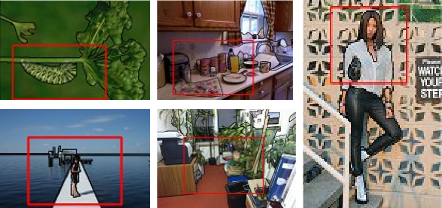
Figure 2 (click to enlarge): Example images from the datasets including ground truth (black boundaries) and excerpts (red boundaries) used for qualitative evaluation, see Qualitative Results. From left top right, top to bottom: BSDS500, NYUV2, SBD, SUNRGBD, Fash.
| BSDS500 | SBD | NYUV2 | SUNRGBD | Fash | |
| Train Images | 100 | 238 | 199 | 200 | 222 |
| Test Images | 200 | 477 | 399 | 400 | 463 |
| Train Size | 481 x 321 | 316 x 240 | 608 x 448 | 658 x 486 | 400 x 600 |
| Test Size | 481 x 321 | 314 x 242 | 608 x 448 | 660 x 488 | 400 x 600 |
Table 2: Number of training and testing images as well as the corresponding average image sizes for each dataset.
Benchmark
The presented core benchmark consists three core evaluation metrics. In the following, let $S = \{S_j\}^K_{j = 1}$ and $G = \{G_i\}$ be partitions of the same image and $I: x_n \rightarrow I(x_n)$, $1 \leq n \leq N$ be an image with $x_n$ being the pixel location and $I(x_n)$ the corresponding intensity or color.
Boundary Recall [40]. Letting $FN(G,S)$ and $TP(G,S)$ be the number of false negative and true positive boundary pixels in $S$ with respect to $G$, Boundary Recall is defined as:
$\text{Rec}(G,S) = \frac{TP(G,S)}{TP(G,S) + FN(G,S)}$
The false negatives and true positives are usually determines using a small tolerance area around individual pixels. Overall, Boundary Recall measures boundary adherence of superpixels.
Undersegmentation Error [3]. Undersegmentation Error quantifies the leakage of superpixels across ground truth segments. The formulation in [45] is computed as
$\text{UE}(G, S) = \frac{1}{N} \sum_{G_i} \sum_{G_i \cap S_j \neq \emptyset} \min \{|S_j \cap G_i|,|S_j - G_i|\}$.
Explained Variation [45]. As ground truth independent measure, Explained Variation quantifies the fraction of image variation that is captured by the superpixel segmentation:
$\text{EV}(G,S) = \frac{\sum_{S_j}|S_j|(\mu(S_j) - \mu(I))^2}{\sum_{x_n}(I(x_n) - \mu(I))^2}$
where $\mu(S_j)$ and $\mu(I)$ are the mean color of superpixel $S_j$ and the image $I$, respectively.
The above metrics inherently depend on the number of generated superpixels $K$. In order to summarize performance of algorithms independent of $K$, $\text{AMR}$, $\text{AUE}$ and $\text{AUEV}$ represent Average Miss Rate, Average Undersegmentation Error and Average Unexplained Variation. These metrics are computed as the area above the $\text{Rec}$ curve, below the $\text{UE}$ curve and above the $\text{EV}$ curve in the range of $[K_\min, K_\max] = [200,5200]$. The names are derived from the Miss Rate $\text{MR} = (1 - \text{Rec})$ and Unexplained Variation $\text{UEV} = (1 - \text{EV})$. Note that in the original version of the paper, these metrics where called Average Boundary Recall $\text{ARec}$ and Average Explained Variation $\text{AEV}$.
Parameter Optimization
Parameter optimization was done using discrete grid search, minimizing $(1 - \text{Rec}) + \text{UE}$ on each dataset individually. Two main challenges made parameter optimization difficult:
- Some superpixel algorithms do not offer control over the number of superpixels, or produce highly varying numbers of superpixels. This, of course, hinders fair comparison. On the one hand, we tried to find simple relationships between parameters and the number of generated superpixels to alleviate the problem for algorithms not providing control over the number of superpixels. On the other hand, we restricted the range of individual parameters in order to ensure that the desired number of superpixels is met within specific bounds. Quantitative examples of both cases can be found in the paper.
- Some implementations are not able to produce connected superpixels. This results in the actual number of superpixels being higher than initially reported and, thus, hinders fair comparison. As solution, we use a connected components algorithms to enforce connectivity across all implementations.
Results
The following two sections briefly summarize some of the main experiments. Detailed discussion can be found in the paper.
The presented visualizations can be found in this GitHub repository. Fullscreen versions are also available: Qualitative Results, Quantitative Results.
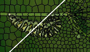
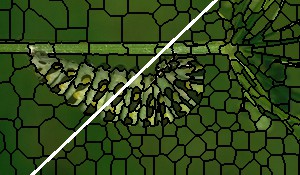
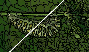
Qualitative
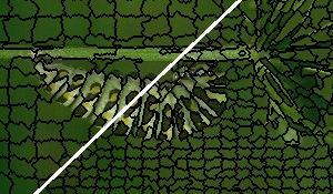
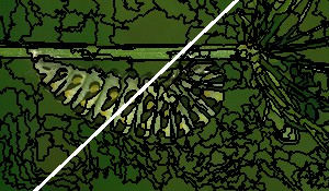
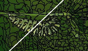
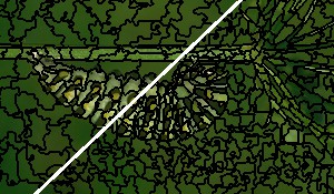
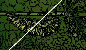
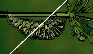
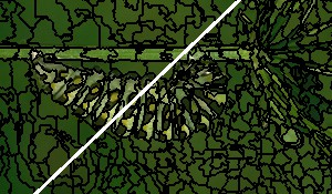
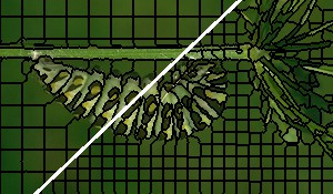
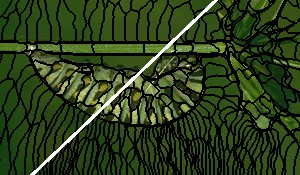
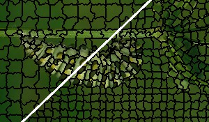
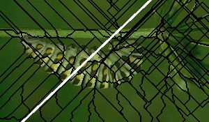
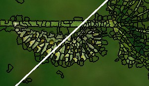
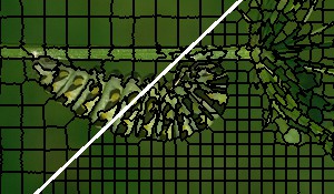
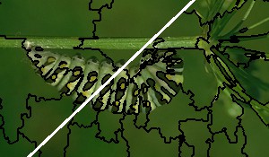
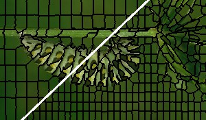
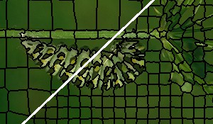
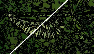
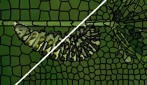
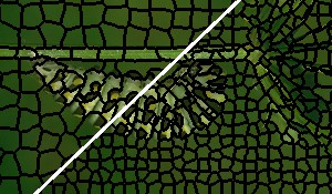
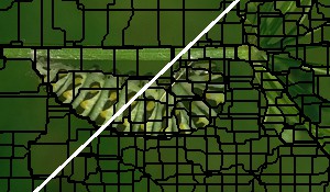
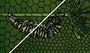
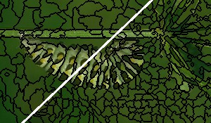
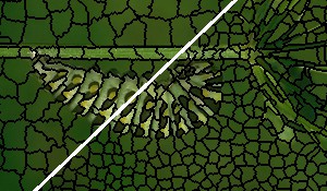
The gallery below shows qualitative results on the BSDS500; specifically, superpixel segmentations for $K \approx 400$ superpixels and $K \approx 1200$ superpixels (top left and bottom right corners, respectively) for each algorithm are shown for an individual image taken from the BSDS500. Also check these Qualitative Results for more examples.
Quantitative
The interactive plots below show $\text{AMR}$, $\text{AUE}$ and $\text{AUEV}$ for all five datasets. Check the same results in fullscreen here.
Ranking
Table 3 shows the final ranking as presented in the paper. The ranking takes into account both $\text{AMR}$ and $\text{AUE}$ reflecting the objective used for parameter optimization. For each algorithm, the table shows the rank distribution across the five datasets.

Table 3 (click to enlarge): Average ranks and rank matrix for all evaluated algorithms. Note that RW, NC and SEAW could not be evaluated on the SUNRGBD dataset and DASP and VCCS cannot be evaluated on the BSDS500, SBD and Fash datasets.
Conclusion
In the paper, we present a large-scale comparison of superpixel algorithms taking into account visual quality, ground truth dependent and independent metrics, runtime, implementation details as well as robustness to noise, blur and affine transformations. For fairness, we systematically optimize parameters while strictly enforcing connectivity. We provide experimental results on five different datasets including indoor, outdoor and person images. We also propose three novel metrics, Average Miss Rate ($\text{AMR}$), Average Undersegmentation Error ($\text{AUE}$) and Average Unexplained Variation ($\text{AUV}$) to summarize algorithm performance independent of the number of generated superpixels. This enables us to present an overall ranking of superpixel algorithms to guide algorithm selection.
Regarding the mentioned aspects of superpixel algorithms, we make the following observatiobns:
- Most algorithms provide good boundary adherence and some algorithms are able to capture small details. However, boundary adherence comes at the cost of reduced compactness, regularity and smoothness. While regularity and smoothness depends on algorithmic details, a compactness parameter allows to trade-off boundary adherence and compactness.
- Performance can be quanitified using well-known metrics such as Boundary Recall, Undersegmentation Error and Explained Variation. However, considering averages of these metrics are not sufficient to discriminate algorithms reliably. Instead, we also consider minimum/maximum as well as standard deviation in order to identifiy stable algorithms — those providing monotonically increasing performance with regard to the number of generated superpixels.
- Several algorithms are able to run in realtime (roughly 30fps); iterative algorithms, in particular, allow to trade performance for runtime.
Acknowledgements
I am grateful for the support of Alexander Hermans and Bastian Leibe. Furthermore, I want to thank all the authors for providing the implementations of their proposed superpixel algorithms. Finally, I acknowledge funding from the EU project STRANDS (ICT-2011-600623).
References
- [1] D. Stutz, A. Hermans, B. Leibe. Superpixels: An Evaluation of the State-of-the-Art. Computing Research Repository, abs/1612.01601.
- [2] D. Martin, C. Fowlkes, J. Malik. Learning to detect natural image boundaries using local brightness, color, and texture cues. IEEE Transactions on Pattern Analysis and Machine Intelligence 26 (5) (2004) 530-549.
- [3] P. Neubert, P. Protzel. Superpixel benchmark and comparison. In: Forum Bildverarbeitung, 2012.
- [4] F. Meyer. Color image segmentation. International Conference on Image Processing and its Applications, 1992, pp. 303-306.
- [5] D. Comaniciu, P. Meer. Mean shift: A robust approach toward feature space analysis. IEEE Transactions on Pattern Analysis and Machine Intelligence 24 (5) (2002) 603–619.
- [6] X. Ren, J. Malik. Learning a classification model for segmentation. International Conference on Computer Vision, 2003, pp. 10–17.
- [7] P. F. Felzenswalb, D. P. Huttenlocher. Efficient graph-based image segmentation. International Journal of Computer Vision 59 (2) (2004) 167–181.
- [8] L. Grady, G. Funka-Lea. Multi-label image segmentation for medical applications based on graph-theoretic electrical potentials. ECCV Workshops on Computer Vision and Mathematical Methods in Medical and Biomedical Image Analysis, 2004, pp. 230–245.
- [9] L. Grady. Random walks for image segmentation. IEEE Transactions on Pattern Analysis and Machine Intelligence 28 (11) (2006) 1768–1783.
- [10] A. Vedaldi, S. Soatto. Quick shift and kernel methods for mode seeking. European Conference on Computer Vision, Vol. 5305, 2008, pp. 705–718.
- [11] F. Drucker, J. MacCormick. Fast superpixels for video analysis. Workshop on Motion and Video Computing, 2009, pp. 1–8.
- [12] A. Levinshtein, A. Stere, K. N. Kutulakos, D. J. Fleet, S. J. Dickinson, K. Siddiqi. TurboPixels: Fast superpixels using geometric flows. IEEE Transactions on Pattern Analysis and Machine Intelligence 31 (12) (2009) 2290–2297.
- [13] O. Veksler, Y. Boykov, P. Mehrani. Superpixels and supervoxels in an energy optimization framework. European Conference on Computer Vision, Vol. 6315, 2010, pp. 211–224.
- [14] R. Achanta, A. Shaji, K. Smith, A. Lucchi, P. Fua, S. Susstrunk. SLIC superpixels. Tech. rep., Ecole Polytechnique Federale de Lausanne (2010).
- [15] R. Achanta, A. Shaji, K. Smith, A. Lucchi, P. Fua, S. Susstrunk. SLIC superpixels compared to state-of-the-art superpixel methods. IEEE Transactions on Pattern Analysis and Machine Intelligence 34 (11) (2012) 2274–2281.
- [16] R. Mester, C. Conrad, A. Guevara. Multichannel segmentation using contour relaxation: Fast super-pixels and temporal propagation. Scandinavian Conference Image Analysis, 2011, pp. 250–261.
- [17] C. Conrad, M. Mertz, R. Mester, Contour-relaxed superpixels. Energy Minimization Methods. Computer Vision and Pattern Recognition, 2013, pp. 280–293.
- [18] M. Y. Lui, O. Tuzel, S. Ramalingam, R. Chellappa. Entropy rate superpixel segmentation. IEEE Conference on Computer Vision and Pattern Recognition, 2011, pp. 2097–2104.
- [19] Y. Zhang, R. Hartley, J. Mashford, S. Burn. Superpixels via pseudo-boolean optimization. International Conference on Computer Vision, 2011, pp. 1387–1394.
- [20] D. Weikersdorfer, D. Gossow, M. Beetz. Depth-adaptive superpixels. International Conference on Pattern Recognition, 2012, pp. 2087–2090.
- [21] M. van den Bergh, X. Boix, G. Roig, B. de Capitani, L. van Gool. SEEDS: Superpixels extracted via energy-driven sampling. European Conference on Computer Vision, Vol. 7578, 2012, pp. 13–26.
- [22] D. Tang, H. Fu, X. Cao. Topology preserved regular superpixel. IEEE International Conference on Multimedia and Expo, 2012, pp. 765–768.
- [23] H. Fu, X. Cao, D. Tang, Y. Han, D. Xu. Regularity preserved superpixels and supervoxels. IEEE Transactions on Multimedia 16 (4) (2014) 1165–1175.
- [24] J. Wang, X. Wang. VCells: Simple and efficient superpixels using edge-weighted centroidal voronoi tessellations. IEEE Transactions on Pattern Analysis and Machine Intelligence 34 (6)(2012) 1241–1247.
- [25] H. E. Tasli, C. Cigla, T. Gevers, A. A. Alatan. Super pixel extraction via convexity induced boundary adaptation. IEEE International Conference on Multimedia and Expo, 2013, pp. 1–6.
- [26] H. E. Tasli, C. Cigla, A. A. Alatan. Convexity constrained efficient superpixel and supervoxel extraction. Signal Processing: Image Communication 33 (2015) 71–85.
- [27] J. Papon, A. Abramov, M. Schoeler, F. Wörgötter. Voxel cloud connectivity segmentation - supervoxels for point clouds. IEEE Conference on Computer Vision and Pattern Recognition, 2013, pp. 2027–2034.
- [28] P. Neubert, P. Protzel. Compact watershed and preemptive SLIC: on improving trade-offs of superpixel segmentation algorithms. International Conference on Pattern Recognition, 2014, pp. 996–1001.
- [29] P. Buyssens, I. Gardin, S. Ruan. Eikonal based region growing for superpixels generation: Application to semi-supervised real time organ segmentation in CT images. Innovation and Research in BioMedical Engineering 35 (1) (2014) 20–26.
- [30] P. Buyssens, M. Toutain, A. Elmoataz, O. Lézoray. Eikonal-based vertices growing and iterative seeding for efficient graph-based segmentation. International Conference on Image Processing, 2014, pp. 4368–4372
- [31] W. Benesova, M. Kottman. Fast superpixel segmentation using morphological processing. Conference on Machine Vision and Machine Learning, 2014.
- [32] V. Machairas, E. Decencière, T. Walter. Waterpixels: Superpixels based on the watershed transformation. International Conference on Image Processing, 2014, pp. 4343–4347.
- [33] V. Machairas, M. Faessel, D. Cardenas-Pena, T. Chabardes, T. Walter, E. Decencière. Waterpixels. Transactions on Image Processing 24 (11) (2015) 3707–3716.
- [34] J. Yao, M. Boben, S. Fidler, R. Urtasun. Real-time coarse-to-fine topologically preserving segmentation. IEEE Conference on Computer Vision and Pattern Recognition, 2015, pp. 2947–2955.
- [35] Z. Li, J. Chen. Superpixel segmentation using linear spectral clustering. IEEE Conference on Computer Vision and Pattern Recognition, 2015, pp. 1356–1363.
- [36] J. M. R. A. Humayun, F. Li. The middle child problem: Revisiting parametric min-cut and seeds for object proposals. International Conference on Computer Vision, 2015, pp. 1600–1608.
- [37] J. Strassburg, R. Grzeszick, L. Rothacker, G. A. Fink. On the influence of superpixel methods for image parsing. International Conference on Computer Vision Theory and Application, 2015, pp. 518–527.
- [38] O. Freifeld, Y. Li, J. W. Fisher. A fast method for inferring high-quality simply-connected superpixels. International Conference on Image Processing, 2015, pp. 2184-2188.
- [39] J. Shen, Y. Du, W. Wang, X. Li. Lazy random walks for superpixel segmentation. Transactions on Image Processing 23 (4) (2014) 1451-1462.
- [40] P. Arbeláez, M. Maire, C. Fowlkes, J. Malik. Contour detection and hierarchical image segmentation. IEEE Transactions on Pattern Analysis and Machine Intelligence 33 (5), 2011.
- [41] S. Gould, R. Fulton, D. Koller. Decomposing a scene into geometric and semantically consistent regions. International Conference on Computer Vision, 2009.
- [42] N. Silberman, D. Hoiem, P. Kohli, R. Fergus. Indoor segmentation and support inference from RGBD images. European Conference on Computer Vision, 2012.
- [43] S. Song, S. P. Lichtenberg, J. Xiao. SUN RGB-D: A RGB-D scene understanding benchmark suite. IEEE Conference on Computer Vision and Pattern Recognition, 2015.
- [44] K. Yamaguchi, K. M. H, L. E. Ortiz, T. L. Berg. Parsing clothing in fashion photographs. IEEE Conference on Computer Vision and Pattern Recognition, 2012.
- [45] A. P. Moore, S. J. D. Prince, J. Warrell, U. Mohammed, G. Jones. Superpixel lattices. IEEE Conference on Computer Vision and Pattern Recognition, 2008.