RESEARCH
Non-Convex Optimization
iPiano, proposed by Ochs et al., is an iterative optimization algorithm combining forward-backward splitting with an inertial force to tackle composite functions. This page presents an implementation of iPiano in C++ with applications to denoising and image segmentation.
Overview
iPiano tackles problems of the form
$\min_{x \in \mathbb{R}^n} h(x) = \min_{\mathbb{R}^n} f(x) + g(x)$.(1)
Here, $f$ is required to be differentiable, but might be non-convex, while $h$ is required to be convex, but might be non-differentiable.
The implementation is available on GitHub:
iPiano on GitHubThe background is discussed in the detail in the following seminar paper:
Seminar PaperBackground
The following references give a short overview of the mathematical background:
Stay tuned for a C++ implementation and a seminar paper on this topic!
Ochs et al. combine two streams of research in optimization: proximal algorithms, in particular forward-backward splitting, with an inertial term. Specifically, Ochs et al. consider problems of the form
$\min_{x \in \mathbb{R}^n} h(x) = \min_{x \in \mathbb{R}^n}(f(x) + g(x))$.
where $f$ is smooth and $g$ convex. The proposed algorithms is termed iPiano and based on the following iteration scheme:
$x^{(n + 1)} = \text{prox}_{\alpha_n g} \left(x^{(n)} - \alpha_n f(x^{(n)}) + \beta_ n(x^{(n)} - x^{(n - 1)})\right)$
where $x^{(n)}$ denotes the $n$-th iterate and $\alpha_n$ and $\beta_n$ are step size and momentum parameter. The proximal mapping is defined as usual, i.e.
$\text{prox}_{\alpha g}(\hat{x}) := \arg\min_{x \in \mathbb{R}^n} \frac{\|x - \hat{x}\|_2^2}{2} + \alpha g(x)$,
and well-defined as $g$ is convex. The algorithm can be summarized as in Algorithm 1 where the interesting part - choosing $\alpha_n$ and $\beta_n$ in order to guarantee convergence - is omitted. Ochs et al. prove convergence for bounded, coercive $h$ where $f$ is smooth (but might be non-convex) and $g$ is proper closed convex (but might be non-smooth). Additional requirements include the Lipschitz-continuity of $\nabla f$ as well as the lower semi-continuity of $g$.
function ipiano(
        $f$, $g$,
        $N$ // Maximum number of iterations
    )
    initialize $x^{(0)}$
    $x^{(-1)} := x^{(0)}$
    for $n = 1,\ldots,N$
        choose $\alpha_n$
        choose $\beta_n$
        $x^{(n + 1)} = \text{prox}_{\alpha_n g} \left(x^{(n)} - \alpha_n f(x^{(n)}) + \beta_n(x^{(n)} - x^{(n - 1)})\right)$
    return $x^{(n)}$
Algorithm 1: Simplified iPiano.
Combettes and Pesquet give a thorough introduction/overview of proximal splitting algorithms to solve problems of the form
$\min_{x \in \mathbb{R}^n} f_1(x) + \ldots + f_m(x)$
for $f_1,\ldots,f_m$ convex functions.
For the following discussion, let
$\text{prox}_{\gamma f}(x) := \arg \min_{\hat{x} \in \mathbb{R}^n} f(\hat{x}) + \frac{1}{2\gamma} \|x - \hat{x}\|_2^2$
the proximal mapping for a proper, convex and lower semi-continuous function $f$.
They discuss multiple approaches including forward-backward splitting applied to the following problem: For $m = 2$, let $f_1$ be proper convex and lower-semi-continuous and $f_2$ be proper and differentiable with $L$-Lipschitz continuous gradient $\nabla f_1$ (note the similarity to the problem considered by Ochs et al. in [1]). Furthermore, $f_1 + f_2$ is required to be coercive, i.e. for $\|x\| \rightarrow \infty$ it is $f_1(x) + f_2(x) \rightarrow \infty$. For this problem, it can be shown that at least one solution exists and the following fix point equation can be derived:
$x^\ast = \text{prox}_{\gamma f_1}(x^\ast - \gamma \nabla f_2(x^\ast))$.
This formulation suggests the following iterative optimization scheme:
$x^{(n + 1)} = \text{prox}_{\gamma_n f_1}(x^{(n)} - \gamma_n \nabla f_2(x^{(n)}))$
where $x^{(n)}$ denotes the $n$-th iterate and $\gamma_n$ the learning rate in the $n$-th iteration. Here, the application of the proximal mapping $\text{prox}_{\gamma_n f_1}$ is called the backward step and $x^{(n)} - \gamma_n \nabla f_2(x^{(n)})$ is called the forward step. The convergence of this approach is obviously depending on the chosen learning rate $\gamma_n$. For Algorithms 1 and 2, convergence has been shown (in [2] and [3], respectively.
function constant_step_forward_backward(
        $f_1$, $f_2$,
        $L$ // Lipschitz constant of $\nabla f_2$
    )
    choose $\epsilon \in (0, \frac{3}{4})$
    initialize $x^{(0)}$
    for $n = 1,\ldots$
        choose $\lambda_n \in [\epsilon, \frac{3}{2} - \epsilon]$
        $x^{(n + 1)} = x^{(n)} + \lambda_n(\text{prox}_{L^{-1} f_1}(x^{(n)} - L^{-1} \nabla f_2(x^{(n)})) - x^{(n)})$
Algorithm 1: Constant-step forward-backward algorithm.
function forward_backward(
        $f_1$, $f_2$,
        $L$ // Lipschitz constant of $\nabla f_2$
    )
    choose $\epsilon \in (0, \min\{1, \frac{1}{L}\})$
    initialize $x^{(0)}$
    for $n = 1,\ldots$
        choose $\gamma_n \in [\epsilon, \frac{2}{L} - \epsilon]$
        choose $\lambda_n \in [\epsilon, \frac{3}{2} - \epsilon]$
        $x^{(n + 1)} = x^{(n)} + \lambda_n(\text{prox}_{\gamma_n f_1}(x^{(n)} - \gamma_n \nabla f_2(x^{(n)})) - x^{(n)})$
Algorithm 2: Forward-backward algorithm.
The forward-backward splitting algorithm can also be generalized to $f_2$ not being convex and an additional inertial force can be integrated as done by Ochs et al. [1]. While Combettes and Pesquet do not discuss signal processing or computer vision applications, Ochs et al. apply their variant of forward-backward splitting to image denoising and image compression.
Beneath the discussion of popular proximal splitting algorithms, Combettes and Pesquet also give an exhaustive list of proximal mappings for various, commonly used functions as well as useful properties of the proximal mapping operator, some of which are summarized in Table 1.
Table 1: Useful properties of the proximal mapping operator.
| Property | $f(x)$ | $\text{prox}_{f}$ |
|---|---|---|
| Translation | $\phi(x - z)$, $z \in \mathbb{R}^n$ | $z + \text{prox}_\phi(x - z)$ |
| Scaling | $\phi(\frac{x}{\rho})$, $\rho \neq 0$ | $\rho\text{prox}_{\frac{\phi}{\rho^2}}(\frac{x}{\rho}$ |
| Reflection | $\phi(-x)$ | $-\text{prox}_\phi(-x)$ |
- [1] P. Ochs, Y. Chen,T. Brox, T. Pock. iPiano: Inertial Proximal Algorithm for Non-Convex Optimization. Computing Research Repository, abs/1404.4805, 2014.
- [2] H. H. Bauschke, P. L. Combettes. Convex Analysis and Monotone Operator Theory in Hilbert Sapces. Springer, 2011.
- [3] P. L. Combettes, V. R. Wajs. Signal Recovery by Proximal Forward-Backward Splitting. Multiscale Model. Simul. 4, 2005.
Shen discusses an approximation to the Mumford-Shah segmentation model [1]:
$h(O, x_+, c_-, u^{(0)}) ) \int_O (u^{(0)}(x) - c_+)^2 dx + \int_{\Omega\setminus O} (u^{(0)}(x) - c_-)^2 dx + \lambda \text{per}(O)$
where $u^{(0)} : \Omega \rightarrow [0,1]$ is an image (for simplicity, let $u^{(0)}$ be a grayscale image) and $O \subset \Omega$ refers to the foreground. Furthermore, $\lambda$ is a regularization parameter and $c_+$/$c_-$ is the average foreground/background intensity. The perimeter $\text{per}(O)$ of $O$ is defined using the total variation of its characteristic function:
$\text{per}(O) := |\chi_O|_{BV(\Omega)}$.
Obviously, minimization over the set $O$ is problematic. One of the most popular approaches to this problem is the work by Chan and Vese [2] who apply the level set framework to minimize over a $3$-dimensional curve instead of the set $O$. Instead, Shen derives a $\Gamma$-convergence formulation of the reduced Mumford-Shah model:
$h_\epsilon (u; c_+, c_-, u^{(0)}, \lambda) = \lambda \underbrace{\int_\Omega \left(9 \epsilon \|\nabla u(x)\|_2^2+ \frac{(1 - u(x)^2)^2}{64 \epsilon}\right) dx}_{= f_\epsilon(u)}$
$+ \int_\Omega \left(\frac{1 + u(x)}{2}\right)^2 (u^{(0)} (x) - c_+)^2 dx + \int_\Omega\left(\frac{1 - u(x)}{2}\right)^2 (u^{(0)} - c_-)^2 dx$
As discussed by Shen, $f_\epsilon(u)$ is used to approximate the perimeter $\text{per}(O)$. To minimize Equation (1), Shen uses an alternative scheme, i.e. for fixed $c_+$ and $c_-$ minimize $h_\epsilon$ and for fixed $u$ compute
$c_+ = \frac{\int_\Omega (1 + u(x))^2 u^{(0)}(x) dx}{\int_\Omega (1 + u(x))^2 dx}$;
$c_- = \frac{\int_\Omega (1 - u(x))^2 u^{(0)}(x) dx}{\int_\Omega (1 - u(x))^2 dx}$.
- [1] D. Mumford, J. Shah. Optimal approximations by piecewise smooth functions and associated variational problems. Comm. on Pure and Applied Mathematics, 42, 1989.
- [2] L. A. Vese, T. F. Chan. A multiphase level set framework for image segmentation using the mumford and shah model. International Journal of Computer Vision, 50, 2002.
Documentation and Examples
Doxygen documentation can be found here. Examples are provided in the repository. Figure 1 shows example results when using iPiano for segmentation as proposed in [2] and compressive sensing (see [3] for an introduction).
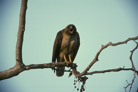
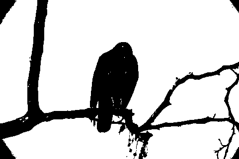


Figure 1 (click to enlarge): Examples illustrating applications of iPiano: segmentation using an approximation to the Mumford-Shah model [2] and recovering sparse signals (original signal on the left; recovered signal on the right) as requred in compressive sensing [3].
Algorithm
iPiano is based on the following iterative scheme:
$x^{(n + 1)} = \text{prox}_{\alpha_n g} (x^{(n)} - \alpha_n \nabla f(x^{(n)}) + \beta_n (x^{(n)} - x^{(n - 1)})$(2)
where $\alpha_n$ is the step size parameter and $\beta_n$ is the momentum parameter in the $n$-th iteration. $\text{prox}_{\alpha_n g}$ denotes the proximal mapping of of $\alpha_n g$ and $\nabla f$ the gradient of $f$. Obviously, the key lies in choosing appropriate $\alpha_n$ and $\beta_n$ in order to guarantee convergence. In the following, the two implemented variants of iPiano are discussed.
nmiPiano. In order to choose $\alpha_n$ appropriately, the Lipschitz constant $L$ of $\nabla f$ needs to be known (or estimated). nmiPiano, presented in Algorithm 1, uses backtracking to estimate $L$ locally in each iteration. In particular, given $x^{(n)}$ and $x^{(n + 1)}$, the estimate $L_n$ is required to satisfy
$f(x^{(n + 1)}) \leq f(x^{(n)}) + \nabla f(x^{(n)})^T(x^{(n + 1)} - x^{(n)}) + \frac{L_n}{2}\|x^{(n + 1)} - x^{(n)}\|_2^2$.(3)
In practice, $x^{(n + 1)}$ is re-estimated until a$L_n \in \{L_{n - 1}, \eta L_{n - 1}, \eta^2 L_{n - 1}, \ldots \}$
is found satisfying Equation (3). nmiPiano adapts $\alpha_n$ according to the estimated $L_n$ while keeping $\beta_n$ fixed.
function constant_step_forward_backward(
        $g$, $f$,
        $L$ // Lipschitz constant of $\nabla f$
    )
    choose $\beta \in [0, 1)$
    choose $L_{- 1} > 0$
    choose $\eta > 1$
    initialize $x^{(0)}$
    for $n = 1,\ldots$
        $L_n := \frac{1}{\eta} L_{n - 1}$ // Initial estimate of $L_n$
        repeat
            $L_n := \eta L_n$ // Next estimate of $L_n$
            choose $\alpha_n < \frac{2(1 - \beta)}{L_n}$
            $\hat{x}^{(n + 1)} = \text{prox}_{\alpha_n g} (x^{(n)} - \alpha_n \nabla f(x^{(n)}) + \beta (x^{(n)} - x^{(n - 1)}))$
        until (3) is satisfied with $\hat{x}^{(n + 1)}$
        $x^{(n + 1)} := \hat{x}^{(n + 1)}$
Algorithm 1 (nmiPiano): iPiano with constant momentum parameter.
iPiano. Algorithm 2, called iPiano, adapts both $\alpha_n$ and $\beta_n$ based on the current estimate $L_n$ of the local Lipschitz constant. Additionally, auxiliary variables $\delta_n$, $\gamma_n$ and constants $c_1$, $c_2$ (close to zero) are introduced in order to bound suitable $\alpha_n$ and $\beta_n$. Specifically, $\alpha_n \geq c_1$ and $\beta_n$ are chosen such that
$\delta_n := \frac{1}{\alpha_n} - \frac{L_n}{2} - \frac{\beta_n}{2\alpha_n} \geq \gamma_n := \frac{1}{\alpha_n} - \frac{L_n}{2} - \frac{\beta_n}{\alpha_n} \geq c_2$.
Then, it can be shown that $\delta_n$ is monotonically decreasing. This, in turn, is required to prove convergence, see [1] for details.
function constant_step_forward_backward(
        $g$, $f$,
        $L$ // Lipschitz constant of $\nabla f$
    )
    choose $L_{- 1} > 0$
    choose $\eta > 1$
    initialize $x^{(0)}$
    for $n = 1,\ldots$
        $L_n := \frac{1}{\eta} L_{n - 1}$ // Initial estimate of $L_n$
        repeat
            $L_n := \eta L_n$ // Next estimate of $L_n$
            repeat
                choose $\alpha_n \geq c_1$
                choose $\beta_n \geq 0$
                $\delta_n := \frac{1}{\alpha_n} - \frac{L_n}{2} - \frac{\beta_n}{2\alpha_n}$
                $\gamma_n := \frac{1}{\alpha_n} - \frac{L_n}{2} - \frac{\beta_n}{\alpha_n}$
            until $\delta_n \geq \gamma_n \geq c_2$
            $\hat{x}^{(n + 1)} = \text{prox}_{\alpha_n g} (x^{(n)} - \alpha_n \nabla f(x^{(n)}) + \beta_n (x^{(n)} - x^{(n - 1)}))$
        until (3) is satisfied with $\hat{x}^{(n + 1)}$
        $x^{(n + 1)} := \hat{x}^{(n + 1)}$
Algorithm 2 (iPiano): iPiano.
References
- [1] P. Ochs, Y. Chen,T. Brox, T. Pock. iPiano: Inertial Proximal Algorithm for Non-Convex Optimization. Computing Research Repository, abs/1404.4805, 2014.
- [2] J. Shen. Gamma-Convergence Approximation to Piecewise Constant Mumford-Shah Segmentation. International Conference on Advanced Concepts for Intelligent Vision Systems, 2005.
- [3] G. Kutyniok. Theory and Applications of Compressed Sensing. Computing Research Repository, abs/1203.3815, 2012.