During the summer term 2015 and the winter term 2015/2016, Prof. Berkels held two lectures on mathematical image processing - in particular, on "Foundations of Mathematical Image Processing" and "Variational Methods in Image Processing". Both lectures included several programming assignments. This article contains some of these exercises including implementations in MatLab and C++.
The source code is available on GitHub:
GitHubThe theoretical background as well as algorithms have been discussed in class. Unfortunately the corresponding lecture notes are in German and not publicly available. However, these methods can be found in most textbooks on image processing and computer vision such as [1] (also in German and close to the lecture) or [2]:
- [1] K. Bredies, D. Lorenz. Mathematische Bildverarbeitung. Vieweg+Teubner, 2011.
- [2] D. Forsyth, P. Jean. Computer Vision: A Modern Approach. Prentice Hall, 1st Edition, 2003.
Histogram Equalization
Task. Implement histogram equalization for grayscale images.
Results are shown in Figure 1.

Filters
Task. Implement the following filters: average/box filter, Gaussian filter, Binomial filter and median filter.
Of course, recent computer vision libraries such as OpenCV offer highly optimized implementations of (linear) filters, but everyone studying computer vision should have implemented some basic filters from scratch.
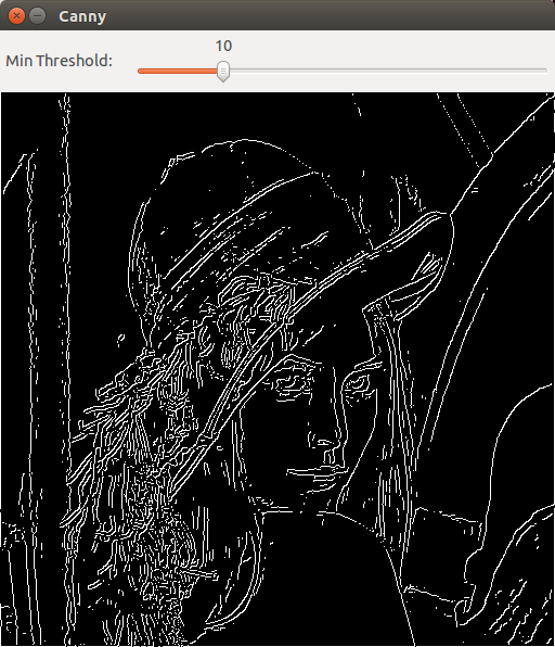
Canny Edges
Task. Implement Canny edges (without hysteresis thresholding and non-maximum suppression).
Results are shown in Figure 2.
Erosion/Dilation and IsoData
Task. Implement erosion, dilation and the isodata algorithm.
Results are shown in Figure 3.

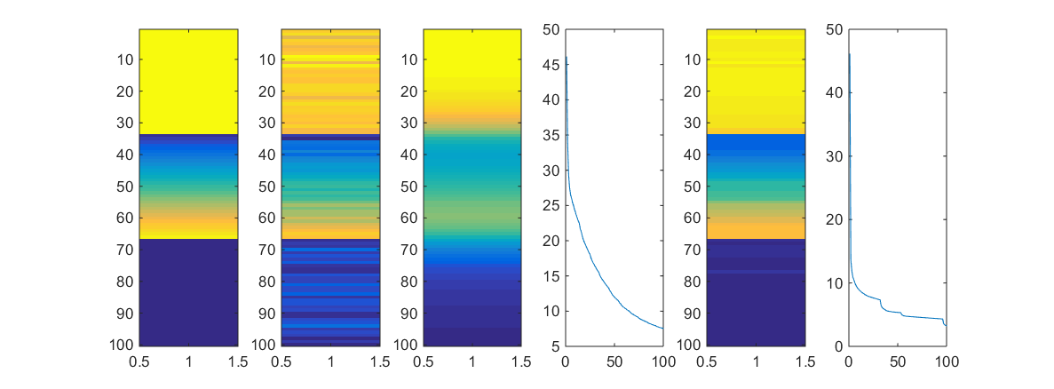
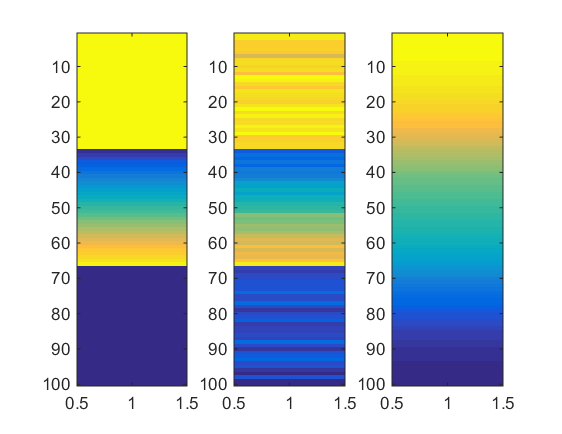
Gradient Descent/Flows for Denoising
Task (Part 1). Implement gradient descent using the Armijo rule for controlling the step size. Use the implementation to denoise one-dimensional signals by minimizing the following functionals:
$J_a(x) = \sum_{i = 1}^n (x_i - f_i)^2 + \lambda \sum_{i = 1}^{n - 1} (x_{i + 1} - x_i)^2$,
$J_b(x) = \sum_{i = 1}^n (x_i - f_i)^2 + \lambda \sum_{i = 1}^{n - 1} |x_{i + 1} - x_i|_\epsilon$
where $x, f \in \mathbb{R}^n$ and $|t|_\epsilon = \sqrt{t^2 + \epsilon^2}$.
Task (Part 2). The minimizer of $J_a$ can uniquely be identified with the solution to a linear system of equations. Implement the minimization procedure of $J_a$ by means of solving a system of linear equations.
Applied on one-dimensional signals, results are shown in Figure 4; in particular, gradient descent produces better results than formulating the problem as system of linear equations. Furthermore, using $J_b$ is able to preserve edges.