This article could also be titled "Struggling with Torch and LUA for Deep Learning". Especially when coming from a Python background, Lua seems like a weird language where all the useful libraries (NumPy, SciPy, etc.) are traded for Torch instead.
In the following, I want to provide examples illustrating common use cases in deep learning research. A rough outline is given on the left. The examples will be developed incrementally, however, can also be considered individually. I start with a few comments on installation and useful packages. The examples can also be found on GitHub:
Torch Examples on GitHubImportant steps in the examples are highlighted and discussed in the text — look out for comments indicating step numbers such as (1), (2), (3), ...
Installation
Installation, following the Getting Started with Torch guide, is easy:
$ git clone https://github.com/torch/distro.git torch-master --recursive
$ cd torch-master
$ bash install-deps
$ ./install.sh
Make sure to restart the console or source ~/.bashrc afterwards. The installation can be tested by running th in the console:
$ th
  ______             __   |  Torch7
 /_  __/__  ________/ /   |  Scientific computing for Lua.
  / / / _ \/ __/ __/ _ \  |  Type ? for help
 /_/  \___/_/  \__/_//_/  |  https://github.com/torch
                          |  http://torch.ch
iTorch
Although the examples in this article are all stand-alone and do not require an iPython/Jupyter notebook, iTorch might come in handy. Assuming that iPython/Jupyter are already installed:
# Dependencies:
$ sudo apt-get install libzmq3-dev libssl-dev python-zmq
$ sudo apt-get install luarocks
$ luarocks install lzmq
# iTorch:
$ git clone https://github.com/facebook/iTorch.git iTorch-master
$ cd iTorch-master
$ luarocks make
Run jupyter to make sure that the Torch kernel is found.
Packages
Two packages that will be discussed in the Utilities examples are torch-hdf5 and luajson:
# luajson
$ git clone https://github.com/harningt/luajson.git luajson-master
$ cd luajson-master
$ luarocks install rockspecs/luajson-1.3.4-1.rockspec
# torch-hdf5
$ sudo apt-get install libhdf5-serial-dev hdf5-tools
$ git clone https://github.com/deepmind/torch-hdf5 torch-hdf5-master
$ cd torch-hdf5-master
$ luarocks make hdf5-0-0.rockspec
Additionally, for some utilities, I found luafilesystem useful:
$ luarocks install luafilesystem
IDE
I found ZeroBrane Studio to be a good IDE to start with LUA and Torch. In order to run Torch from within ZeroBrane, the following steps are helpful:
- Download the Torch plugin from here and save it to
~/.zbstudio/packages. - Set
export TORCH_BIN=/path/to/torch-master/install/bin/thin.bashrc. - Start ZeroBrane from console using
zbstudio.
Getting Started
To get started, we consider the example from the documentation illustrating a simple 2-dimensional classification task:
-- Simple 2D classification example taken somewhere from the Torch docs.
-- Uses the nn.StochasticGradient trainer.

require('torch')
require('nn')

-- (1) Setup the dataset, nn.StochasticGradient requires a :size() method.
dataset = {}
function dataset:size()
  return 100
end

-- (2) The dataset should contain inputs and outputs (targets) such that dataset[i][0]
-- is the input of sample i and dataset[i][0] the corresponding outputs.
for i = 1, dataset:size() do
  local input = torch.randn(2)
  local output = torch.Tensor(1)
  if input[1]*input[2] > 0 then
    output[1] = -1;
  else
    output[1] = 1
  end
  dataset[i] = {input, output}
end

-- (3) Setup a simple classifier by adding the corresponding layers
-- to a nn.Sequential container.
model = nn.Sequential()
model:add(nn.Linear(2, 20))
model:add(nn.Tanh())
model:add(nn.Linear(20, 1))

-- (4) nn.StochasticTrainer expects a model and a criterion (here the MSECriterion)
-- for training.
learningRate = 0.01
criterion = nn.MSECriterion()
trainer = nn.StochasticGradient(model, criterion)
trainer.learningRate = learningRate
trainer:train(dataset)
nn.StochasticGradient.This example uses nn.StochasticGradient for training — for getting started, this is appropriate, however later examples will show that using optim is more flexible. Let us go through the individual steps of :
nn.StochasticGradientrequires a dataset implementing thesizemethod returning the overall number of samples.- The dataset provides inputs and outputs/targets such that
dataset[i][0]is the input of sample i anddataset[i][1]the corresponding output. nn.Sequentialis a container allowing to easily build feed-forward networks by sequentially adding layers/operations; in this example, a simple classifier is defined.- For training, a criterion is required; in this case, we use a mean squared error objective.
While simple, the example can easily be extended by considering real-world datasets — check lua-csv, torch/image or torch-hdf5 for useful packages. It also allows to define more complex models by considering different containers and the large catalog of layers, activation functions and criteria.
Training an Auto-Encoder
Instead of the simple classification example in Listing , I want to work on a more flexible auto-encoder example — maybe because data generation is trivial for auto-encoders. The following listing shows how to train a shallow auto-encoder using nn.StochasticGradient:
-- Simple auto-encoder example.
-- Uses the nn.StochasticGradient trainer.

require('math')
require('torch')
require('nn')

N = 1000
D = 100

dataset = {}
function dataset:size()
  return N
end

-- (1) The dataset will contain vectors of ones and the task
-- will be to denoise these vectors; more complex datasets are easily implemented.
for i = 1, dataset:size() do
  local output = torch.ones(D)
  local input = torch.cmul(output, torch.randn(D)*0.05 + 1)
  dataset[i] = {input, output}
end

-- (2) Setup a simple auto-encoder with bottleneck.
model = nn.Sequential()
model:add(nn.Linear(D, D/2))
model:add(nn.Tanh())
model:add(nn.Linear(D/2, D))

-- (3) Change the criterion to an absolute difference criterion.
learningRate = 0.01
criterion = nn.AbsCriterion()
trainer = nn.StochasticGradient(model, criterion)
trainer.learningRate = learningRate
trainer:train(dataset)
nn.StochasticGradient.Listing is analogously to Listing except that we train a denoising auto-encoder:
- As dataset, we want to denoise simple vectors filled with one.
- The model changes to a simple auto-encoder with bottleneck.
- As criterion, the absolute difference is used.
For real-world data and more complex models, nn.StochasticGradient is fairly limited — also because of the strict expectations regarding the dataset. In the following, I will gradually move to using optim for training.
Training using updateParameters
In order to provide more flexibility regarding the dataset (for example control over the batch size, shuffling, on-the-fly data augmentation), Module.updateParameters can be used for gradient descent training. This is illustrated in Listing :
-- Auto-encoder example adapted from the Torch docs.

require('math')
require('torch')
require('nn')

N = 1000
D = 100

-- (1) Setup the dataset; note that the dataset is not bound to
-- the structure used for nn.StochasticTraining anymore.
inputs = torch.Tensor(N, D)
outputs = torch.Tensor(N, D)

for i = 1, N do
  outputs[i] = torch.ones(D)
  inputs[i] = torch.cmul(outputs[i], torch.randn(D)*0.05 + 1)

  if i%100 == 0 then
    print('[Data] '..i)
  end
end

model = nn.Sequential()
model:add(nn.Linear(D, D/2))
model:add(nn.Tanh())
model:add(nn.Linear(D/2, D))

-- (2) Setup the batch size, learning rate and the
-- absolute difference criterion.
batchSize = 10
learningRate = 0.01
criterion = nn.AbsCriterion()

-- (3) The main loop defining the number of iterations.
for i = 1, 500 do
  -- (3.1) Input and output batch is chosen randomly from the dataset.
  -- This is done by shuffling the indices and selecting a fixed subset.
  local shuffle = torch.randperm(N)
  shuffle = shuffle:narrow(1, 1, batchSize)
  shuffle = shuffle:long()

  local input = inputs:index(1, shuffle)
  local output = outputs:index(1, shuffle)

  -- (3.2) Forward pass of the network and the criterion.
  local loss = criterion:forward(model:forward(input), output)

  -- (3.3) Zero the accumulated gradients.
  model:zeroGradParameters()
  -- (3.4) Compute gradients for this iteration using a backward pass
  -- of the criterion and the model.
  model:backward(input, criterion:backward(model.output, output))
  -- (3.5) Update the parameters using a gradient descent step.
  model:updateParameters(learningRate)

  print('[Training] '..i..': '..loss)
end
Module.updateParameters.Dataset and model are the same as in Listing . However, instead of using nn.StochasticGradient, Module.updateParameters is used for gradient descent training where the batches are chosen randomly:
- Here, dataset is not bound to the restrictions when using
nn.StochasticGradient; thus, inputs and outputs are handled separately allowing to easily draw random batches. - As criterion, the absolute difference is used; and the batch size is set.
- In the main training loop, a gradient descent step is performed on a random batch:
- The batch is chosen randomly by shuffling the corresponding indices.
- The network output and loss are computed using a forward pass of the network and the criterion, respectively.
- Before computing the gradients, the accumulated gradients of the last iterations are set to zero.
- The gradients are then computed using a backward pass of the criterion and the network.
- Finally, the parameters are updated using a gradient descent steps with the given learning rate.
Training using Module.updateParameters is still inflexible regarding the optimization procedure — it is bound to gradient descent and cannot be monitored easily. In the next example we will finally using optim for training.
Training using optim
optim is Torch's numeric optimization package and includes many standard optimization algorithms — for example stochastic gradient, AdaGrad, AdaDelta, Adam and many more. It allows to define the objective to minimize as local function and step through optimization iteration by iteration. Of course, this involves a few more lines of code, however, is also flexible regarding the objective — for example for including weight decay as shown in Listing :
-- Simple auto-encoder example.
-- Uses optim (https://github.com/torch/optim) for training.

require('math')
require('torch')
require('nn')
require('optim')

N = 10000
D = 100

inputs = torch.Tensor(N, D)
outputs = torch.Tensor(N, D)

for i = 1, N do
  outputs[i] = torch.ones(D)
  inputs[i] = torch.cmul(outputs[i], torch.randn(D)*0.05 + 1)

  if i%100 == 0 then
    print('[Data] '..i)
  end
end

model = nn.Sequential()
model:add(nn.Linear(D, D/2))
model:add(nn.Tanh())
model:add(nn.Linear(D/2, D))

-- (1) In addition to batch size and learning rate, we additionally
-- define a momentum parameter and the weight decay weight.
batchSize = 10
learningRate = 0.01
momentum = 0.9
weightDecay = 0.05
criterion = nn.AbsCriterion()

-- (2) Get the parameters and its gradients on which to perform stochastic
-- gradient descent. Note that there are some caveats with getParameters:
-- https://github.com/torch/DEPRECEATED-torch7-distro/issues/33
parameters, gradParameters = model:getParameters()

T = 2500
for t = 1, T do

  -- Sample a random batch from the dataset.
  local shuffle = torch.randperm(N)
  shuffle = shuffle:narrow(1, 1, batchSize)
  shuffle = shuffle:long()

  local input = inputs:index(1, shuffle)
  local output = outputs:index(1, shuffle)

  -- (3) Define the objective function, called feval.
  --- Definition of the objective on the current mini-batch.
  -- This will be the objective fed to the optimization algorithm.
  -- @param x input parameters
  -- @return object value, gradients
  local feval = function(x)

    -- Get new parameters.
    if x ~= parameters then
      parameters:copy(x)
    end

    -- (3.1) As before, reset the accumulated gradients.
    gradParameters:zero()

    -- (3.2) Compute the forward pass of the network and the criterion.
    local pred = model:forward(input)
    local f = criterion:forward(pred, output)

    -- (3.3) Estimate the gradients through a backward pass of the
    -- network and criterion.
    local df_do = criterion:backward(pred, output)
    model:backward(input, df_do)

    -- (3.4) Add weight decay if requested.
    if weightDecay > 0 then
      f = f + weightDecay * torch.norm(parameters,2)^2/2
      gradParameters:add(parameters:clone():mul(weightDecay))
    end

    return f, gradParameters
  end

  sgdState = sgdState or {
      learningRate = learningRate,
      momentum = momentum
  }

  -- (4) Run optim.sgd for one step on the defined objective.
  -- The parameters and the objective value is returned.
  p, f = optim.sgd(feval, parameters, sgdState)

  print('[Training] '..t..': '..f[1])
end
optim.Let us go through Listing step by step:
- In addition to the learning rate and batch size,
optimeasily allows us to add a momentum term and weight decay; the criterion remains unchanged. - For optimization, the parameters and gradient tensors are obtained from the network using
Module.getParameters. - The objective function is a function of the parameters and returns the function value as well as its gradients at the given parameter point; the steps within the objective are similar to Listing :
- First, the gradient parameters from the last iteration are set to zero.
- Network output/predictions and the loss are computed using a forward pass.
- The gradients are computed using a backward pass.
- A weight decay term is added if the weight is greater than zero.
optim.sgdtakes the objective function, the current parameters and the current state.
The example in Listing is very flexible regarding the objective as well as the optimization algorithms. More criteria can be found in the catalog of criteria and can also be combined using nn.MultiCriterion or nn.ParallelCriterion. More optimization algorithms can be found in the optim docs. We will also see an example of a custom criterion later.
GPU Training
Recent advances in deep learning are powered by the latest graphics cards. Thus, Torch allows to easily train models with GPU acceleration through packages such as cutorch and cunn. The following example illustrates how to adapt Listing to leverage GPU acceleration:
-- Simple auto-encoder example.
-- Uses optim (https://github.com/torch/optim) and GPU for training.

require('math')
require('torch')
require('nn')
require('optim')
require('cunn')

N = 10000
D = 100

inputs = torch.Tensor(N, D)
outputs = torch.Tensor(N, D)

for i = 1, N do
  outputs[i] = torch.randn(D)
  inputs[i] = torch.cmul(outputs[i], torch.randn(D)*0.05 + 1)

  if i%100 == 0 then
    print('[Data] '..i)
  end
end

model = nn.Sequential()
model:add(nn.Linear(D, 3*D))
model:add(nn.Tanh())
model:add(nn.Linear(3*D, D))
-- (1) Convert to model.
model = model:cuda()

batch_size = 10
learning_rate = 0.01
momentum = 0.9
weight_decay = 0.05

criterion = nn.AbsCriterion()
-- (2) Convert the criterion.
criterion = criterion:cuda()

parameters, gradParameters = model:getParameters()
-- (3) Convert the parameters and their gradients.
parameters = parameters:cuda()
gradParameters = gradParameters:cuda()

T = 2500
for t = 1, T do

  -- Sample a random batch from the dataset.
  local shuffle = torch.randperm(N)
  shuffle = shuffle:narrow(1, 1, batch_size)
  shuffle = shuffle:long()

  local input = inputs:index(1, shuffle)
  local output = outputs:index(1, shuffle)

  -- (4) Convert input and output.
  input = input:cuda()
  output = output:cuda()

  --- Definition of the objective on the current mini-batch.
  -- This will be the objective fed to the optimization algorithm.
  -- @param x input parameters
  -- @return object value, gradients
  local feval = function(x)

     -- Get new parameters.
     if x ~= parameters then
        parameters:copy(x)
     end

     -- Reset gradients
     gradParameters:zero()

     -- Evaluate function on mini-batch.
     local pred = model:forward(input) -- pred will be CUDA Tensor
     local f = criterion:forward(pred, output)

     -- Estimate df/dW.
     local df_do = criterion:backward(pred, output)
     model:backward(input, df_do)

     -- weight decay
     if weight_decay > 0 then
        f = f + weight_decay * torch.norm(parameters,2)^2/2
        gradParameters:add(parameters:clone():mul(weight_decay))
     end

     -- return f and df/dX
     return f, gradParameters
  end

  sgdState = sgdState or {
      learningRate = learning_rate,
      momentum = momentum,
      learningRateDecay = 5e-7
  }

  -- Returns the new parameters and the objective evaluated
  -- before the update.
  p, f = optim.sgd(feval, parameters, sgdState)

  print('[Training] '..t..': '..f[1])
end
optim and GPU acceleration provided by cunn.For successfully using cunn to accelerate training, four steps are required:
- Convert the network to CUDA.
- Convert to criterion to CUDA.
- Convert the parameters and the gradients to CUDA.
- And convert the input and output for each foward/backward pass to CUDA.
Overall, it is very easy to adapt examples to use GPU acceleration. Therefore, in the following, most examples will work without CUDA.
Convolutional Auto-Encoder
The following example is based on Listing but trains a convolutional auto-encoder to remove salt and pepper noise from a white rectangle in the middle of an image:
-- Convolutional auto encoder example.

require('torch')
require('nn')
require('optim')
require('lfs')

N = 1000
C = 1
H = 8 -- divisible by four
W = 8 -- divisible by four

inputs = torch.Tensor(N, C, H, W)
outputs = torch.Tensor(N, C, H, W)

for i = 1, N do
  -- (1) A binary image with a white square in the middle is
  -- generated and salt and pepper noise is added.
  outputs[i] = torch.Tensor(C, H, W):fill(0)
  outputs[i]:sub(1, 1, H/2 - 2, H/2 + 2, W/2 - 2, H/2 + 2):fill(1)
  inputs[i] = outputs[i]

  -- Random indices to set 0.
  zeroIndices = torch.Tensor(C, H, W):uniform():mul(1.05):floor()
  inputs[i][zeroIndices:eq(1)] = 0

  oneIndices = torch.Tensor(C, H, W):uniform():mul(1.05):floor()
  inputs[i][oneIndices:eq(1)] = 1
end

-- (1) The convolutional auto-encoder follows the general design in the
-- literature and is analogous to non-convolutional auto-encoders.
-- It consists of an encoder, a bottleneck (the code) and a decoder.
-- (1.1) The encoder applies spatial convolutions and max pooling
-- to reduce the feature map size.
model = nn.Sequential()
model:add(nn.SpatialConvolutionMM(1, 8, 3, 3, 1, 1, 1, 1))
model:add(nn.ReLU(true))
model:add(nn.SpatialMaxPooling(2, 2, 2, 2))
model:add(nn.SpatialConvolutionMM(8, 8, 3, 3, 1, 1, 1, 1))
model:add(nn.ReLU(true))
model:add(nn.SpatialMaxPooling(2, 2, 2, 2))

-- (1.2) The last feature map is now resized to a vector
-- using nn.View. The number of units is simultaneously the
-- dimensionality of the code.
hidden = H/4*W/4*8
model:add(nn.View(hidden))
model:add(nn.Linear(hidden, hidden))
model:add(nn.ReLU(true))

-- (1.3) The decode starts by reshaping the linear input
-- and then applies upsampling and convolutions to reconstruct
-- the input.
model:add(nn.View(8, H/4, W/4))
model:add(nn.SpatialUpSamplingNearest(2))
model:add(nn.SpatialConvolutionMM(8, 8, 3, 3, 1, 1, 1, 1))
model:add(nn.ReLU(true))
model:add(nn.SpatialUpSamplingNearest(2))
model:add(nn.SpatialConvolutionMM(8, 1, 3, 3, 1, 1, 1, 1))
model:add(nn.ReLU(true))

batchSize = 10
learningRate = 0.01
momentum = 0.9
weightDecay = 0.05
criterion = nn.AbsCriterion()

parameters, gradParameters = model:getParameters()

T = 2500
for t = 1, T do

  -- Sample a random batch from the dataset.
  local shuffle = torch.randperm(N)
  shuffle = shuffle:narrow(1, 1, batchSize)
  shuffle = shuffle:long()

  local input = inputs:index(1, shuffle)
  local output = outputs:index(1, shuffle)

  --- Definition of the objective on the current mini-batch.
  -- This will be the objective fed to the optimization algorithm.
  -- @param x input parameters
  -- @return object value, gradients
  local feval = function(x)

     -- Get new parameters.
     if x ~= parameters then
        parameters:copy(x)
     end

     -- Reset gradients
     gradParameters:zero()

     -- Evaluate function on mini-batch.
     local pred = model:forward(input)
     local f = criterion:forward(pred, output)

     -- Estimate df/dW.
     local df_do = criterion:backward(pred, output)
     model:backward(input, df_do)

     -- weight decay
     if weightDecay > 0 then
        f = f + weightDecay * torch.norm(parameters,2)^2/2
        gradParameters:add(parameters:clone():mul(weightDecay))
     end

     -- return f and df/dX
     return f, gradParameters
  end

  sgdState = sgdState or {
      learningRate = learningRate,
      momentum = momentum,
      learningRateDecay = 5e-7
  }

  -- Returns the new parameters and the objective evaluated
  -- before the update.
  p, f = optim.sgd(feval, parameters, sgdState)

  print('[Training] '..t..': '..f[1])
end
optim.The only two differences compared to Listing is the data generation and the network architecture:
- As toy data, binary images with a white square in the middle are generated and salt and pepper noise is applied.
- The model is a convolutional auto-encoder as known from the literature; it consists of an encoder and a decoder:
- The encoder takes the input images and applies convolutional and max pooling layers to subsample the input by factor four.
- The subsampled feature maps are reshaped using
nn.Viewand a linear layer is applied; although the dimensionality is not reduced further, this is the bottleneck. - The decoder starts by reshaping the code using
nn.Viewand using nearest neighbor upsampling and convolutional layers to reconstruct the input — hopefully with less noise.
Although this example is comparably simple, it illustrates the general pieces needed to train convolutional neural networks. A useful insight, for example, is that Torch works with the dimensions (batch, channels, height, width) — using a different ordering might result in problems with individual layers. Based on this minimal example, more complex convolutional networks can be constructed by consulting the catalog of convolutional layers.
Weight Initialization
Weight initialization is governed by Module.reset which takes as optional argument the standard deviation $\sigma$ to be used for initialization. Weights and biases are then drawn from a uniform distribution in $(-\sigma,\sigma)$. This allows to manually initialize the weights and biases using most of the well-known initialization schemes. The following listing shows a simple package adapted from e-lab/torch-toolbox:
-- Adapted from https://github.com/e-lab/torch-toolbox/blob/master/Weight-init/weight-init.lua.
require("nn")

-- (1) Define several initialization schemes; these compute, given
-- the number of input and output units the standard deviation
-- to be used for Module.reset.

--- Initialization scheme introduced in
-- "Efficient backprop", Yann Lecun, 1998
-- @param fanIn number of input units
-- @param fanOut number of output units
-- @return standard deviation to use
local function initHeuristic(fanIn, fanOut)
  return math.sqrt(1/(3*fanIn))
end

--- Initialization scheme introduced in
-- "Understanding the difficulty of training deep feedforward neural networks", Xavier Glorot, 2010
-- @param fanIn number of input units
-- @param fanOut number of output units
-- @return standard deviation to use
local function initXavier(fanIn, fanOut)
  return math.sqrt(2/(fanIn + fanOut))
end

--- Initialization scheme introduced in
-- "Delving Deep into Rectifiers: Surpassing Human-Level Performance on ImageNet Classification", Kaiming He, 2015
-- @param fanIn number of input units
-- @param fanOut number of output units
-- @return standard deviation to use
local function initKaiming(fanIn, fanOut)
  return math.sqrt(4/(fanIn + fanOut))
end

--- Use the given method to initialize all layers.
-- @param model model to initialize
-- @param methodName method to use
-- @return model
local function init(model, methodName)
  methodName = methodName or 'xavier'

  local method = nil
  if methodName == 'heuristic' then
    method = initHeuristic
  elseif methodName == 'xavier' then
    method = initXavier
  elseif methodName == 'kaiming' then
    method = initKaiming
  else
    assert(false)
  end

  -- (2) Go through all modules and apply the chosen initialization scheme
  -- to layers with weights and biases.
  for i = 1, #model.modules do
    local m = model.modules[i]
    if m.__typename == 'nn.SpatialConvolution' then
      m:reset(method(m.nInputPlane*m.kH*m.kW, m.nOutputPlane*m.kH*m.kW))
    elseif m.__typename == 'nn.SpatialConvolutionMM' then
      m:reset(method(m.nInputPlane*m.kH*m.kW, m.nOutputPlane*m.kH*m.kW))
    elseif m.__typename == 'nn.Linear' then
      m:reset(method(m.weight:size(2), m.weight:size(1)))
    end

    if m.bias then
      m.bias:zero()
    end
  end

  return model
end

return init
The approach for initialization using Module.reset is simple:
- Different initialization methods such as
initHeuristicandinitXavierare defined, each expecting the number of input and output units in order to compute the standard deviation forModule.reset. - The
initfunction loops over all modules and applies the initialization function to layers with weights and biases.
The package provided in Listing is easily used as follows:
model = nn.Sequential()
-- Add more layers.
init = require('init') -- Assumes the package to be saved in init.lua
model = init(model, 'xavier')
However, the code in Listing still relies on Module.reset — which, for example, initializes weights and biases in a similar manner. More control can be obtained by directly initializing weights and biases. The following listing shows how to access the weights and biases of a module directly; for example to initialize the baises to zero:
-- A more complex initialization module which allows non-uniform initialization
-- not using the layers' reset method.
require("nn")

-- (1) The initialization methods now take the tensor
-- to be initialized (weights or biases) and an optional
-- value in addition to fan in and fan out.

--- Initialize a tensor with a fixed value.
-- @param tensor tensor to initialize
-- @param fanIn number of input units
-- @param fanOut number of output units
-- @param value value to initialize with
local function initFixed(tensor, fanIn, fanOut, value)
  if tensor then
    tensor:fill(value)
  end
end

--- Uniform initialization.
-- @param tensor tensor to initialize
-- @param fanIn number of input units
-- @param fanOut number of output units
-- @param value value to use as range for uniform intialization
local function initUniform(tensor, fanIn, fanOut, value)
  if tensor then
    tensor:uniform(-value, value)
  end
end

--- Initialize a tensor according to normal distribution.
-- @param tensor tensor to initialize
-- @param fanIn number of input units
-- @param fanOut number of output units
-- @param value value to initialize with
local function initNormal(tensor, fanIn, fanOut, value)
  if tensor then
    tensor.normal(0, value)
  end
end

--- Initialization scheme introduced in
-- "Efficient backprop", Yann Lecun, 1998
-- @param tensor tensor to initialize
-- @param fanIn number of input units
-- @param fanOut number of output units
-- @param value not used
local function initHeuristic(tensor, fanIn, fanOut, value)
  local std = math.sqrt(1/(3*fanIn))
  std = std * math.sqrt(3)

  if tensor then
    tensor:uniform(-std, std)
  end
end

--- Initialization scheme introduced in
-- "Understanding the difficulty of training deep feedforward neural networks", Xavier Glorot, 2010
-- @param tensor tensor to initialize
-- @param fanIn number of input units
-- @param fanOut number of output units
-- @param value not used
local function initXavier(tensor, fanIn, fanOut, value)
  local std = math.sqrt(2/(fanIn + fanOut))
  std = std * math.sqrt(3)

  if tensor then
    tensor:uniform(-std, std)
  end
end

--- Initialization scheme introduced in
-- @param tensor tensor to initialize
-- @param fanIn number of input units
-- @param fanOut number of output units
-- @param value not used
local function initKaiming(tensor, fanIn, fanOut, value)
  local std = math.sqrt(4/(fanIn + fanOut))
  std = std * math.sqrt(3)

  if tensor then
    tensor:uniform(-std, std)
  end
end

--- Get the init function by its name.
-- @param name name of the function
-- @return the function
local function getMethodByName(name)
  if name == 'fixed' then
    return initFixed
  elseif name == 'uniform' then
    return initUniform
  elseif name == 'normal' then
    return initNormal
  elseif name == 'heursitic' then
    return initHeuristic
  elseif name == 'xavier' then
    return initXavier
  elseif name == 'kaiming' then
    return initKaiming
  else
    assert(false)
  end
end

--- Use the given method to initialize all layers.
-- @param model model to initialize
-- @param methodName method to use
-- @return model
local function init(model, weightsMethodName, weightsValue, biasMethodName, biasValue)

  local weightsValue = weightsValue or 0.05
  local biasMethodName = biasMethodName or 'fixed'
  local biasValue = biasValue or 0.0

  -- (3) Different initialization schemes for weights and biases.
  local weightsMethod = getMethodByName(weightsMethodName)
  local biasMethod = getMethodByName(biasMethodName)

  -- (2) Loop over all modules and separately initialize weights and biases.
  -- Depending on the chosen initialization method, the optional value can or cannot be used.
  for i = 1, #model.modules do
    local m = model.modules[i]
    if m.__typename == 'nn.SpatialConvolution' then
      weightsMethod(m.weight, m.nInputPlane*m.kH*m.kW, m.nOutputPlane*m.kH*m.kW, weightsValue)
      biasMethod(m.bias, m.nInputPlane*m.kH*m.kW, m.nOutputPlane*m.kH*m.kW, biasValue)
    elseif m.__typename == 'nn.SpatialConvolutionMM' then
      weightsMethod(m.weight, m.nInputPlane*m.kH*m.kW, m.nOutputPlane*m.kH*m.kW, weightsValue)
      biasMethod(m.bias, m.nInputPlane*m.kH*m.kW, m.nOutputPlane*m.kH*m.kW, biasValue)
    elseif m.__typename == 'nn.Linear' then
      weightsMethod(m.weight, m.weight:size(2), m.weight:size(1), weightsValue)
      biasMethod(m.bias, m.weight:size(2), m.weight:size(1), biasValue)
    end
  end

  return model
end

return init
Listing differs from Listing only in that initialization is applied separately to weights and biases. In addition, initialization is not done through Module.reset:
- The initialization methods now expect the tensor to be initialized and an optional value in addition to the number of input and output units.
- Different initialization schemes for weights and biases can be used.
- In the loop over all modules, the two initialization methods are applied to weights and biases separately.
Usage of Listing changes to:
model = init(model, 'xavier', 0, 'fixed', 0) -- Initialize weights using Xavier and biases to zero.
Weight Visualization
torch/gnuplot provides basic plotting capabilities for Torch. A simple example of visualizing the weight matrices of a model as trained in Listing is given below:
require('gnuplot')
require('torch')
require('nn')

-- (1) Assumes the models has been saved using
-- torch.save to 'model.bin' in the same directory.
modelFile = 'model.bin'
model = torch.load(modelFile)

-- Comment this out to print all modules
-- and get the corresponding indices.
--for i = 1, #model.modules do
--  print(model.modules[i])
--end

-- (2) Plot the weight matrices as images using
-- gnuplot.imagesc.
-- (2.1) The weights of the first layer.
gnuplot.pngfigure('linear1.png')
gnuplot.imagesc(model.modules[1].weight, 'color')
gnuplot.plotflush()

-- (2.2) The weights of the second layer.
gnuplot.pngfigure('linear3.png')
gnuplot.imagesc(model.modules[3].weight, 'color')
gnuplot.plotflush()
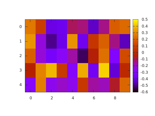
The example is comparably simple; one of the main insights is using model.modules[i] to access the $i$-th module. Some comments:
- The model is assumed to be saved in
model.bin— saving and loading models is also discussed in Saving and Loading Models. gnuoplot.imagescis used to plot a weight matrix as shown in Figure .
Admittedly, the example in Listing is very simple and torch/gnuplot provides more examples for plotting. However, I still prefer to use the power of Python and matplotlb to produce fancy visualizations. As we will see in Utilities it is easy to use Python for plotting and post-processing using the HDF5 format for data exchange.
Extensions
Torch is easy to extend — simply consulting carpedm20/awesome-torch will lead to many interesting repositories implementing the latest networks from research. However, the most common cases will include writing custom criteria and custom modules (i.e. layers).
Criteria
Custom criteria are easily implemented by extending nn.Criterion. Listing shows a custom implementation of nn.AbsCriterion.
require('torch')
require('nn')

-- (1) Small helper function to compute the normalization used
-- in CustomAbsCriterion.
--- Compute the product of elements in a storage.
-- @param storage storage to compute product of
-- @return product of all dimensions
local function storageProd(storage)
  local prod = 1
  for i = 1, #storage do
    prod = prod * storage[i]
  end
  return prod
end

-- (2) Extend nn.Criterion, the newly created criterion is called
-- CustomAbsCriterion and accessible as nn.CustomAbsCriterion after
-- requiring this file.
--- @class CustomAbsCriterion
local CustomAbsCriterion, parent = torch.class('nn.CustomAbsCriterion', 'nn.Criterion')

--- Initialize the criterion.
function CustomAbsCriterion:__init()
   parent.__init(self)
end

-- (3) The forward pass of the criterion, i.e.
-- given inputs and targets, compute the loss.
--- Update/compute output given input and target.
-- @param input input computed by the network
-- @param target target to compute loss on
function CustomAbsCriterion:updateOutput(input, target)
  local norm = storageProd(#input)
  self.output = 1/norm*torch.sum(torch.abs(input - target))
  return self.output
end

-- (4) The backward pass of the criterion, i.e.
-- given original inputs and targets, compute the
-- derivative with respect to the inputs.
--- Update the gradients with respect to the input.
-- @param input input computed by the network
-- @param target target to compute loss on
function CustomAbsCriterion:updateGradInput(input, target)
  self.gradInput:resizeAs(input)
  local difference = input - target
  local norm = storageProd(#input)
  self.gradInput[difference:lt(0)] = -1/norm
  self.gradInput[difference:gt(0)] = 1/norm
  return self.gradInput
end
nn.AbsCriterion, i.e. $\sum_i |o_i - t_i|$ where $o_i$ are the network outputs and $t_i$ are the corresponding targets.The following steps are necessary to define a new criterion (in most cases; more complex criteria might require more work):
- The first step is specific to the
CustomAbsCriterion; it is a helper function to compute the product of elements in a storage container — this is used in steps (3) and (4) to compute the normalization term. - The
CustomAbsCriterionis defined here; it directly extendsnn.Criterionand will (after requiring the definition) be available asnn.CustomAbsCriterion. - The forward pass of the criterion is computed in the
updateOutputfunction; it expects the network outputs and the targets. Note that additional arguments (or less arguments for unsupervised criteria) are possible. Intermediate results can also be saved for the backward pass. - Corresponding to the forward pass in
updateOutput, the backward pass is defined inupdateGradInput. It computes the gradients of the criterion with respect to the inputs.
The example in Listing is very flexible. As mentioned above, the number of parameters for updateOutput and updateGradInput can be adapted and are then mirrored by forward and backward. This allows to implement unsupervised, semi-supervised and supervised criteria as well as combine inputs from different models or layers.
Using nn.CustomAbsCriterion is straight-forward. For example, changing Listing to include:
criterion = nn.CustomAbsCriterion()
nn.CustomAbsCriterion usage. For example, in Listing , this is the only line that needs to be changed.A criterion definition can also rely on already implemented criteria; a good example is nn.CrossEntropyCriterion which internally relies on nn.ClassNLLCriterion. A criterion could also contain its own network.
Modules
Implementing a new module is similar to implementing criteria — modules extend nn.Module, however, also implement updateOutput and updateGradInput. The following listing shows the implementation of a PCA projection as custom module. Note that this example assumes that PCA has already been performed (i.e. the matrix $V$ and the mean $\mu$ are pre-computed; then the operation is defined as $y = V(x - \mu)$ — quite similar to a general linear layer):
-- (1) Define the layer, extend from nn.Module.
-- The layer will be accessible via nn.PCA.
--- @class PCA
local PCA, PCAParent = torch.class('nn.PCA', 'nn.Module')

-- (2) The constructor can take arbitrary input parameters.
--- Required constructor.
-- @param W weight matrix
-- @param b bias vector
function PCA:__init(W, b)
  PCAParent.__init(self)
  -- (2.1) If layers have parameters, they should use self.weight and self.bias.
  -- Then the parameters are accessible via :getParameters() and the usage
  -- is consistent across layers.
  -- This also holds if the parameters are not learned, i.e. not adapted
  -- during training.
  self.weight = W
  self.bias = b
end

-- (3) The updateOutput method computes the forward pass of the layer.
-- The input will be the output of the previous layer and, thus,
-- may have different dimensions.
--- Compute output of layer.
-- @param intput input tensor
-- @return output
function PCA:updateOutput(input)
  if input:dim() == 2 then
    -- (3.1) Below is a simple implementation of V*(input - mean):
    local centered = input:t() - torch.repeatTensor(self.bias, input:size(1), 1):t()
    self.output = torch.mm(self.weight:t(), centered)
    self.output = self.output:t()
    return self.output
  else
    assert(false)
  end
end

-- (4) updateGradInput computes the gradients with respect to the inputs
-- by using the gradients from the top layer.
-- In this case, the backward pass is not supported, not implemented.
--- Update gradients with respect to input.
-- @param input input tensor
-- @param gradOutputs gradient outputs from top layer
-- @return gradient with respect to input
function PCA:updateGradInput(input, gradOutput)
  assert(false)
end

-- (5) As the parameters are not trainable, :parameters() is overwritten
-- to return nothing.
--- Overwrite parameters as the fixed weight and bias are not considered
-- trainable parameters.
-- See https://github.com/torch/nn/blob/master/Module.lua#L327 for an
-- error message you will get otherwise
function PCA:parameters()
  return
end

-- (6) As the parameters are not trainable, :accGradParameters
-- is overwritten to do nothing.
-- Usually, it would compute the gradients with respect to
-- self.weight and self.bias and store them in
-- self.gradWeight and self.gradBias, respectively.
--- Avoids accumulating gradient in order to fix the parameters
-- for fine-tuning.
function PCA:accGradParameters(input, gradOutput, scale)
  -- Nothing!
end
Listing may be a non-standard example, but illustrates many important points. Let us go through the listing step by step:
nn.PCAextendsnn.Module.- It takes two arguments, the weight matrix
Wand the mean vectorb. To follow all other modules, these are saved inself.weightandself.bias. These are the variables considered by the:parameters()and:getParameters()methods. In case a module extends existing modules other thannn.Module(e.g. ann.PCA-similar module could extendnn.Linear),PCAParent.__initrefers to the parent's constructor. - The
updateOutputmethod computes the forward pass of the module. In this case:self.weight*(input - self.bias)is computed, corresponding to $V(x - \mu)$. Also note that the rank of the input is checked explicitly.
updateGradInputis used to compute the gradients with respect to the input. It expects the original input and the gradients of the top layer and is supposed to setself.gradInputand return it. In this example,nn.PCAdoes not support a backward pass. In this case, a simple assert ensures thatbackwardcannot be called.- As
nn.PCAdoes not have trainable parameters, theparametersmethod is overwritten. This is good practice as it prevents the parameters (and its gradients) to be included in the flattened parameters returned by:getParameters(). - Similarly, the
accGradParametersmethod is overwritten. Usually, this method would take the original input, the gradients of the top layer to compute the the gradients with respect to the weights, saved inself.gradWeight, and with respect to the biases, saved inself.gradBias.
While the above examples shows how very flexible modules can be defined, the best blueprint is provided by nn.Linear implementing all the necessary methods as discussed above. More examples will also be discussed in Fixing Weights.
Fixing Biases and Weights
For pre-training and fine-tuning, it might be useful to fix weights and biases. First, the trivial case of fixing biases to zero is discussed, then different strategies for fixing the weights are discussed.
Fixing Biases
A closer look at some of the basic modules such as nn.Linear or nn.SpatialConvolution reveals that they provide a :noBias() method. This could for example be used as in Listing . However, it also shows that setting bias and gradBias to nil may also be sufficient.
--- Calls noBias on all modules supporting to disable the bias.
-- @param model model to fix the biases for
function fixBiases(model)
  for i = 1, #model.modules do
    if model.modules[i].__typename == 'nn.Linear' or model.modules[i].__typename == 'nn.SpatialConvolution' then
      model.modules[i]:noBias()
    end
    -- Might need manually adding additional layers that support noBias, this is not a comprehensive list!
  end
end
noBias to fixing the biases to zero.Fixing Weights
For fixing weights, there is no such method as noBias. Instead, Listing shows that when overwriting accGradParameters, it is possible to manually set the weights and keep them fixed during training.
--- Sets all layers with parameters (weights or biases) to be fixed, i.e. overwrites
-- the parameters function to return nothing and the accGradParameters function to
-- to nothing. Should be applied before getParameters is called!
-- @param model model to fix the given layers
-- @param layers indices of layers to fix.
function utils.fixLayers(model, layers)
  for i = 1, #layers do
    if model.modules[layers[i]].weight ~= nil or model.modules[layers[i]].bias ~= nil then

      -- Set gradients to nil for clarity.
      if model.modules[layers[i]].weight ~= nil then
        model.modules[layers[i]].gradWeight:fill(0)
      end
      if model.modules[layers[i]].bias ~= nil then
        model.modules[layers[i]].gradBias:fill(0)
      end

      -- Has no trainable parameters.
      model.modules[layers[i]].parameters = function() end
      -- Does not compute gradients w.r.t. parameters.
      model.modules[layers[i]].accGradParameters = function(input, gradOutput, scale) end
      -- Note that updateGradInput is not touched!
    end
  end
end
Fine Tuning
Listing shows how to fix the weights after manually setting them. This is, for example, useful after loading a saved model as described in Loading and Saving Models. In this case, the model does not change it structure, i.e. the model is loaded, some layers are fixed and it might be fine-tuned on additional data. However, this does not cover the case where the structure of the network changes. Then, the workflow might be as follows: a trained model is loaded, a slightly different model is created and the weights of specific layers are copied (and maybe fixed). Then, the new model is fine-tuned. Listing shows the missing part, i.e. copying weights.
--- Copies the weights of the given layers between two models; assumes the layers to have .weight and .bias defined.
-- @param modelFrom mode to copy weights from
-- @param modelTo model to copy weights to
-- @param layersFrom layer indices in model_from
-- @param layersTo layer indices in model_to
function utils.copyWeights(modelFrom, modelTo, layersFrom, layersTo)
  assert(#layersFrom == #layersTo)

  for i = 1, #layersFrom do
    assert(modelFrom.modules[layersFrom[i]].__typename == modelTo.modules[layersTo[i]].__typename,
        'layer from ' .. layersFrom[i] .. ' and layer to ' .. layersTo[i] .. ' are not of the same type!')

    -- Allows to provide all layers, also these without parameters.
    if modelTo.modules[layersTo[i]].weight ~= nil then
      modelTo.modules[layersTo[i]].weight = modelFrom.modules[layersFrom[i]].weight:clone()
      modelTo.modules[layersTo[i]].gradWeight:resize(#modelFrom.modules[layersFrom[i]].gradWeight)
    end
    if modelTo.modules[layersTo[i]].bias ~= nil then
      modelTo.modules[layersTo[i]].bias = modelFrom.modules[layersFrom[i]].bias:clone()
      modelTo.modules[layersTo[i]].gradBias:resize(#modelFrom.modules[layersFrom[i]].gradBias)
    end
  end
end
A complete example of using Listing as well as the discussion in Fixing Biases and Weights is shown below:
-- Example of fine-tuning where weights obtained forman
-- auto-encoder are fixed, and an additional fully connected
-- layer is then trained for classification.

require('torch')
require('nn')
require('optim')

-- (1) LinearFT extends nn.Linear to overwrite accGradParameters
-- in order to fix both weights and biases.
--- @class LinearFT
local LinearFT, LinearFTParent = torch.class('nn.LinearFT', 'nn.Linear')

--- Required constructor.
-- @param inputSize number of input units
-- @param outputSize number of output units
-- @param bias whether to use a bias
function LinearFT:__init(inputSize, outputSize, bias)
  LinearFTParent.__init(self, inputSize, outputSize, bias)
end

--- Avoids accumulating gradient in order to fix the parameters
-- for fine-tuning.
function LinearFT:accGradParameters(input, gradOutput, scale)
  -- Nothing!
end

-- (2) A simple, unsafe method for copying weights.
-- This version does not check the module types.
--- "Unsafe": Copies the weights of the given layers between two models; does not check
-- that the layers are of the same type; assumes the layers to have .weight and .bias defined.
-- @param modelFrom mode to copy weights from
-- @param modelTo model to copy weights to
-- @param layersFrom layer indices in model_from
-- @param layersTo layer indices in model_to
function copyWeights(modelFrom, modelTo, layersFrom, layersTo)
  assert(#layersFrom == #layersTo)

  for i = 1, #layersFrom do
    modelTo.modules[layersTo[i]].weight = modelFrom.modules[layersFrom[i]].weight
    modelTo.modules[layersTo[i]].bias = modelFrom.modules[layersFrom[i]].bias
  end
end

-- Set up a dataset which will be used for training or testing.
N = 10000
D = 100

batchSize = 10
learningRate = 0.01
momentum = 0.9
weightDecay = 0.05

-- (3) The example should be run twice; first, an auto-encoder
-- is trained, then this model is fien tuned for classification.
modelFile = 'model.dat'
if utils.fileExists(modelFile) then

  -- Classification dataset.
  inputs = torch.Tensor(N, D)
  outputs = torch.Tensor(N, 1)
  line = torch.rand(D)

  for i = 1, N do
    inputs[i] = torch.rand(D)
    outputs[i] = inputs[i]:dot(line)

    if outputs[i][1] > 0 then
      outputs[i][1] = 1
    else
      outputs[i][1] = 0
    end
  end

  trainedModelLayers = {1, 3}
  modelLayers = {1, 3}

  -- (4) The model for classification fixes the second linear layer of the
  -- auto-encoder using LinearFT.
  -- Define the model.
  model = nn.Sequential()
  model:add(nn.Linear(D, D/5)) -- check that weights change due to LinearFT!
  model:add(nn.Tanh())
  model:add(nn.LinearFT(D/5, D/10))
  model:add(nn.Tanh())
  model:add(nn.Linear(D/10, 1))
  model:add(nn.Sigmoid())
  model = init(model, 'xavier')

  -- (5) The auto-encoder is loaded and the weights of the first and
  -- second linear layers are copied.
  -- The remaining part for training is similar to the other
  -- examples.
  trainedModel = torch.load(modelFile)
  -- Copy weights without checking the layer types!
  copyWeights(trainedModel, model, trainedModelLayers, modelLayers)

  criterion = nn.BCECriterion()
  parameters, gradParameters = model:getParameters()

  T = 2500
  for t = 1, T do

    -- Sample a random batch from the dataset.
    local shuffle = torch.randperm(N)
    shuffle = shuffle:narrow(1, 1, batchSize)
    shuffle = shuffle:long()

    local input = inputs:index(1, shuffle)
    local output = outputs:index(1, shuffle)

    --- Definition of the objective on the current mini-batch.
    -- This will be the objective fed to the optimization algorithm.
    -- @param x input parameters
    -- @return object value, gradients
    local feval = function(x)

      -- Get new parameters.
      if x ~= parameters then
        parameters:copy(x)
      end

      -- Reset gradients
      gradParameters:zero()

      -- Evaluate function on mini-batch.
      local pred = model:forward(input)
      local f = criterion:forward(pred, output)

      -- Estimate df/dW.
      local df_do = criterion:backward(pred, output)
      model:backward(input, df_do)

      -- weight decay
      if weightDecay > 0 then
        f = f + weightDecay * torch.norm(parameters,2)^2/2
        gradParameters:add(parameters:clone():mul(weightDecay))
      end

      -- return f and df/dX
      return f, gradParameters
    end

    state = state or {
      learningRate = learningRate,
      momentum = momentum,
      learningRateDecay = 5e-7
    }

    -- Returns the new parameters and the objective evaluated
    -- before the update.
    p, f = optim.sgd(feval, parameters, state)
    print('[Training] ' .. t .. ': ' .. f[1])

    -- To check that first layer weights change if using LinearFT as second
    -- layer!
    --print('[Training] '..t..': '..torch.mean(model.modules[1].weight))
  end
else -- Train and save a new model.

  -- Auto-encoder dataset.
  inputs = torch.Tensor(N, D)
  outputs = torch.Tensor(N, D)

  for i = 1, N do
    outputs[i] = torch.ones(D)
    inputs[i] = torch.cmul(outputs[i], torch.randn(D)*0.05 + 1)
  end

  -- Define the model.
  model = nn.Sequential()
  model:add(nn.Linear(D, D/5))
  model:add(nn.Tanh())
  model:add(nn.Linear(D/5, D/10))
  model:add(nn.Tanh())
  model:add(nn.Linear(D/10, D))
  model = init(model, 'xavier')

  criterion = nn.AbsCriterion()
  parameters, gradParameters = model:getParameters()

  T = 2500
  for t = 1, T do

    -- Sample a random batch from the dataset.
    local shuffle = torch.randperm(N)
    shuffle = shuffle:narrow(1, 1, batchSize)
    shuffle = shuffle:long()

    local input = inputs:index(1, shuffle)
    local output = outputs:index(1, shuffle)

    --- Definition of the objective on the current mini-batch.
    -- This will be the objective fed to the optimization algorithm.
    -- @param x input parameters
    -- @return object value, gradients
    local feval = function(x)

      -- Get new parameters.
      if x ~= parameters then
        parameters:copy(x)
      end

      -- Reset gradients
      gradParameters:zero()

      -- Evaluate function on mini-batch.
      local pred = model:forward(input)

      local f = criterion:forward(input, output)

      -- Estimate df/dW.
      local df_do = criterion:backward(pred, output)
      model:backward(input, df_do)

      -- weight decay
      if weightDecay > 0 then
        f = f + weightDecay * torch.norm(parameters,2)^2/2
        gradParameters:add(parameters:clone():mul(weightDecay))
      end

      -- return f and df/dX
      return f, gradParameters
    end

    state = state or {
      learningRate = learningRate,
      momentum = momentum,
      learningRateDecay = 5e-7
    }

    -- Returns the new parameters and the objective evaluated
    -- before the update.
    p, f = optim.sgd(feval, parameters, state)
    print('[Pre-Training] ' .. t .. ': ' .. f[1])
  end

  torch.save(modelFile, model)
  print('Training completed; rerun to test.')
end
The example is very similar to the other examples presented in this article, except that it is meant to be run twice. First an auto-encoder is trained, then the auto-encoder is fine-tuned for classification:
nn.LinearFTcorresponds to an extension ofnn.Linearfixing both biases and weights. As discussed in Fixing Biases and Weights, this is a simple way to define layers that are meant to be fixed for fine-tuning.- The method
copyWeightsis a simpler version of the one presented in Listing that does not check the correct types of the layers. - The example is split into two parts: In the first run, an auto-encoder is trained. In the second run, the auto-encoder is fine-tuned for classification. Here, the first block of code corresponds to the latter, i.e. is executed in the trained auto-encoder has been saved in
model.dat. - The classification network will take both linear layers of the auto-encoder, fix only the second one using
nn.LinearFT, and add an additional layer for classification. - The trained model in
model.datis loaded usingtorch.loadand then the weights are copied from the loaded model to the new one.
Utilities
The following subsections discuss some useful utility functions.
Loading and Saving Models
Loading and saving models is easy:
modelFile = 'model.dat'
model = nn.Sequential()
-- ...
torch.save(modelFile, model)
-- ...
model = torch.load(modelFile)
Although is the simplest option to load and save models, there are some caveats. First, it matters whether a model has been converted to :cuda() or not. So it might be good practice to only save CPU models. Second, the size of the model file might be artifically increased by automatically saving all the temporary data in the modules (see here). This can be avoided as follows:
model = nn.Sequential()
-- Setup the architecture ...
-- Convert to CUDA if necessary ...

parameters, gradParameters = model:getParameters()
-- Get a model of the same structure with shared weights.
saveModel = model:clone('weight','bias')

-- Now do training, after training is complete, save the second model:
modelFile = 'model.dat'
torch.save(modelFile, saveModel)
Reading and Writing HDF5
I found HDF5 to be a good format to load and exchange data — especially as I still tend to pre-process or generate data using Python. An example of reading and writing tensors from and to HDF5 files is shown in Listing . In addition, shows how h5py can be used to provide data using Python.
-- https://github.com/deepmind/torch-hdf5
require('hdf5')

--- Writes a single torch tensor to HDF5.
-- @param file file to write to
-- @param tensor tensor to write
-- @param key optional key, i.e. tensor is accessible as "/key"
function utils.writeHDF5(file, tensor, key)
  local key = key or 'tensor'
  local h5 = hdf5.open(file, 'w')
  h5:write('/' .. key, tensor)
  h5:close()
end

--- Reads a single torch tensor from HDF5.
-- @param file file to read
-- @param key key to read from, i.e. read "/key"
-- @return tensor
function utils.readHDF5(file, key)
  local key = key or 'tensor'
  local h5 = hdf5.open(file, 'r')
  tensor = h5:read('/' .. key):all()
  h5:close()
  return tensor
end
import h5py
import numpy as np

def write_hdf5(file, tensor, key = 'tensor'):
    """
    Write a simple tensor, i.e. numpy array ,to HDF5.

    :param file: path to file to write
    :type file: str
    :param tensor: tensor to write
    :type tensor: numpy.ndarray
    :param key: key to use for tensor
    :type key: str
    """

    assert type(tensor) == np.ndarray, 'file %s not found' % file

    h5f = h5py.File(file, 'w')

    chunks = list(tensor.shape)
    if len(chunks) > 2:
        chunks[2] = 1
        if len(chunks) > 3:
            chunks[3] = 1

    h5f.create_dataset(key, data = tensor, chunks = tuple(chunks), compression = 'gzip')
    h5f.close()

def read_hdf5(file, key = 'tensor'):
    """
    Read a tensor, i.e. numpy array, from HDF5.

    :param file: path to file to read
    :type file: str
    :param key: key to read
    :type key: str
    :return: tensor
    :rtype: numpy.ndarray
    """

    assert os.path.exists(file), 'file %s not found' % file

    h5f = h5py.File(file, 'r')
    tensor = h5f[key][()]
    h5f.close()

    return tensor
JSON for Configuration
JSON is convenient to handle configuration. Listing demonstrates how to read and write JSON files:
-- https://github.com/harningt/luajson
require('json')
--- Write a table as JSON to a file.
-- @param file file to write
-- @param t table to write
function utils.writeJSON(file, t)
  local f = assert(io.open(file, 'w'))
  f:write(json.encode(t))
  f:close()
end

--- Read a JSON file into a table.
-- @param file file to read
-- @return JSON string
function utils.readJSON(file)
  local f = assert(io.open(file, 'r'))
  local tJSON = f:read('*all')
  f:close()
  return json.decode(tJSON)
end
Filesystem
For interactions with the filesystem, luafilesystem proved to be useful. Listing provides some utilities demonstrating the usage; more information can be found in the documentation.
--- Checks if a file exists.
-- @see http://stackoverflow.com/questions/4990990/lua-check-if-a-file-exists
-- @param filePath path to file
-- @return true if file exists
function utils.fileExists(filePath)
  local f = io.open(filePath, 'r')
  if f ~= nill then
    io.close(f)
    return true
  else
    return false
  end
end

--- Checks if a directory exists using the lfs package.
-- @param dirPath path to directory
-- @return true if directory exists
function utils.directoryExists(dirPath)
  local attr = lfs.attributes(dirPath)
  if attr then
    if attr['mode'] == 'directory' then
      return true
    end
  end

  return false
end

--- Reverse a list.
-- @see http://lua-users.org/wiki/ListOperations
-- @param list list ot reverse
-- @return reversed list
function utils.reverseList(list)
  local rList = {}
  for i = table.getn(list), 1, -1 do
    table.insert(rList, list[i])
  end
  return rList
end

--- Recursively create the given directory; not throrougly tested, might be sensitive to non-linux
-- file paths.
-- @param dirPath path to directory
function utils.makeDirectory(dirPath)
  local function findDirectories(subPath, dirCache, i)
    local lastChar = dirPath:sub(subPath:len(), subPath:len())
    if lastChar == '/' then
      subPath = subPath:sub(1, -2)
    end

    if subPath:len() > 0 then
      if not utils.directoryExists(subPath) then
        dirCache[i] = subPath
        -- http://stackoverflow.com/questions/5243179/what-is-the-neatest-way-to-split-out-a-path-name-into-its-components-in-lua
        local subSubPath, subDir, ext = string.match(subPath, "(.-)([^\\/]-%.?([^%.\\/]*))$")
        findDirectories(subSubPath, dirCache, i + 1)
      end
    end
  end

  local dirCache = {}
  findDirectories(dirPath, dirCache, 1)
  local rDirCache = utils.reverseList(dirCache)

  for i = 1, #rDirCache do
    lfs.mkdir(rDirCache[i])
  end
end