Introduction
The existence of adversarial examples is still poorly understood. A recent hypothesis states that adversarial examples are able to fool deep neural networks because they leave the (possibly low-dimensional) underlying manifold of the data. This assumption is supported by recent experiments [] showing that adversarial examples have low probability under the data distribution.
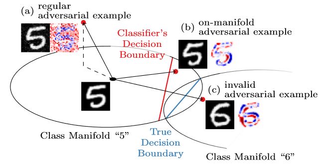
Figure 1: Illustration of the difference between regular, unconstrained adversarial examples and on-manifold adversarial examples as discussed in [].
In my previous post, I outlined how to explicitly constrain adversarial examples to the manifold. On FONTS, a synthetic dataset with known manifold introduced in my recent CVPR'19 paper [], and on MNIST [] using an approximated manifold, these on-manifold adversarial examples result in meaningful manipulation of the image content, as shown in Figure 1. This is in stark contrast to the seemingly random noise patterns of regular, unconstrained adversarial examples. Overall, these experiments further support the hypothesis that adversarial examples leave the underlying data manifold.
In this article, I want to demonstrate that adversarial examples indeed leave the manifold. To this end, given the known or approximated manifold, adversarial examples are projected onto the manifold to show that they exhibit significant distance to the manifold and nearly always leave the manifold in an orthogonal direction. Again, these experiments are taken from my recent CVPR'19 paper [].
Adversarial Examples
Following [], adversarial examples are computed to maximize classificaiton loss. Given an input-label pair $(x,y)$ and a deep neural network $f$, the loss $\mathcal{L}(f(\tilde{x}), y)$ is maximized to obtain the adversarial example $\tilde{x} = x + \delta$. Specifically,
$\max_\delta \mathcal{L}(f(x + \delta), <)$ such that $\|\delta\|_\infty \leq \epsilon$ and $\tilde{x}_i \in [0,1]$(1)
is solved iteratively using projected gradient ascent. This means that after each gradient ascent iteration, the current perturbation $\delta$ is projected back onto the $L_\infty$-ball of radius $\epsilon$ and individual pixel values of $\tilde{x}$ are clipped to $[0,1]$. Optimization can be stopped as soon as $f(x) \neq y$, meaning the label changed. In contrast to the on-manifold adversarial examples, the perturbations $\delta$ are not constrained to be "meaningful". As a result, the perturbations are often seemingly random, see Figure 1.
Distance to Manifold
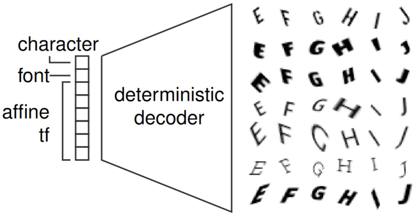
FONTS is a synthetic, MNIST-like datasets containing images of size $28 \times 28$ depicting randomly transformed characters "A" to "J" taken from a diverse set of Google Fonts. Here, the manifold in terms of the used font, the class and the transformation parameters is known. Specifically, let $z$ denots the font, character and affine transformation (shear, scale, translation and rotation), the generative process is modeled using the decoder shown in Figure 2 and detailed in an earlier blog post. Specifically, a prototype image is generated by rendering the given character in the given font and a spatial transformer network applies the affine transformation. As a result, the generative process is differentiable. Thus, given an adversarial example $\tilde{x}$, we can search the latent space for the closest on-manifold example as follows:
$\tilde{z} = \arg\min_z \|\text{dec}(z) - \tilde{x}\|_2$
which can be solved using gradient descent. Then, the distance of $\tilde{x}$ to the manifold is $\|\text{dec}(\tilde{z}) - \tilde{x}\|_2$. As all training/test examples have been generated using the decoder $\text{dec}$, they naturally lie on the manifold — meaning their distance to the manifold is $0$.
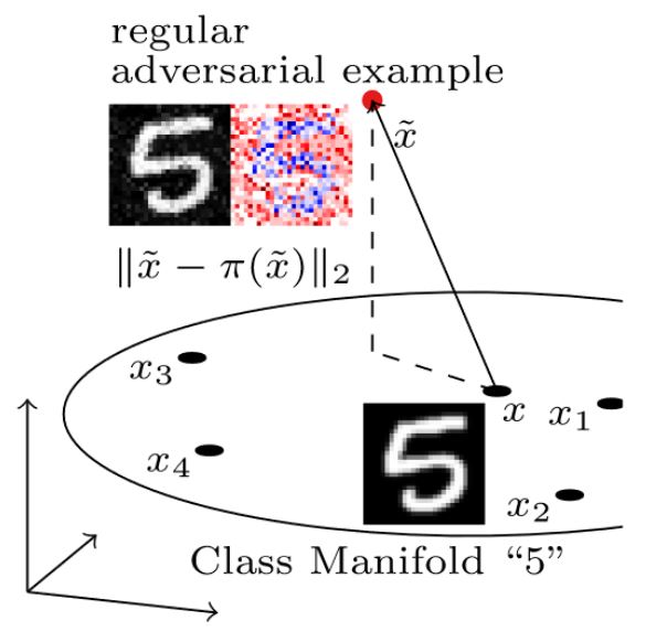
Figure 2: Illustration of the generation process of FONTS, illustrating the underlying, known manifold; using the depicted decoder, adversarial examples can be projected onto the manifold iteratively.
On MNIST, the manifold is not known. However, as illustrated in Figure 3, a simple $k$-nearest neighbor approximation is sufficient. In particular, given an adversarial example $\tilde{x}$ corresponding to the image $x$, the $50$ nearest neighbors $x_1, \ldots, x_50$ of $x$ are found. The adversarial example $\tilde{x}$ is then projected onto the supspace spanned by the vectors $x_i - x$. The projection $\pi(\tilde{x})$ can be computed using least squares allowing to obtain the distance $\|\pi(\tilde{x}) - \tilde{x}\|_2$. In comparison to FONTS, this distance will not be zero even for examples from the manifold, meaning training or test examples. However, the distances can easily be compared to adversarial examples that are constrained to an approximation of the MNIST manifold.
Results
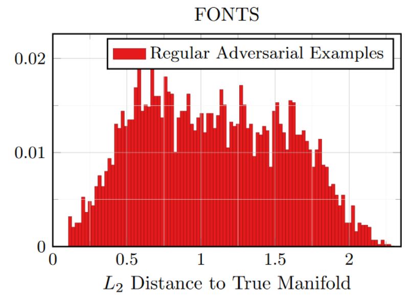
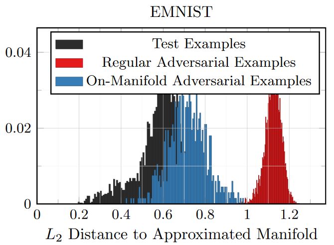
Figure 3: Empirical results on FONTS and MNIST showing the distances of (regular) adversarial examples to the manifold. On MNIST, for comparison, the distances for test and on-manifold adversarial examples are shown, as well.
Figure 3 shows distance histograms on FONTS and MNIST. On FONTS, training/test as well as on-manifold adversarial examples have — by construction — a distance of zero to the manifold. Adversarial examples computed using Equation (1), in contrast, clearly exhibit non-zero distance. Interestingly, the distance to the manifold nearly corresponds to the $L_2$ norm of the perturbations $\delta$. This implies that the direction from $x$ to $\tilde{x} = x + \delta$ is nearly orthogonal with respect to the manifold. On MNIST, the distances of test and on-manifold adversarial examples are added as reference. It can be seen that the distance distribution of on-manifold adversarial examples nearly matches the one of test examples. The difference is mainly due to the approximation of the manifold used to compute on-manifold adversarial examples. Again, "regular" adversarial examples exhibit significantly larger distance, clearly distinguishable from on-manifold adversarial examples and test examples.
Conclusion and Outlook
Overall, this article shows that adversarial examples can be shown to (empirically) leave the underlying manifold of the data — both if the manifold is known and approximated. This means that the observed lack in adversarial robustness might be due to missing guidance of what to compute/how to behave off manifold. In future articles, I will built upon these insights and show how on-manifold adversarial examples can be used to improve generalization — resulting in an approach similar to adversarial data augmentation — and how to potentially improve both robustness and generalization when guiding the network how to behave off manifold.
- [] David Stutz, Matthias Hein, Bernt Schiele. Disentangling Adversarial Robustness and Generalization. CVPR 2019.
- [] Yang Song, Taesup Kim, Sebastian Nowozin, Stefano Ermon, Nate Kushman. PixelDefend: Leveraging Generative Models to Understand and Defend against Adversarial Examples. ICLR (Poster) 2018.
- [] Aleksander Madry, Aleksandar Makelov, Ludwig Schmidt, Dimitris Tsipras, Adrian Vladu. Towards Deep Learning Models Resistant to Adversarial Attacks. ICLR, 2018.
- [] Yann LeCun, Leon Bottou, Yoshua Bengio, and Patrick Haffner. Gradient-based learning applied to documentrecognition. Proceedings of the IEEE, 86(11):2278–2324, 1998.