In deep learning, stochastic gradient descent training usually results in point estimates of the network weights. As such, these estimates can be interpreted as maximum likelihood or maximum a posteriori estimates (potentially given a prior on the weights). Bayesian approaches, in contrast, aim to estimate the posterior distribution over weights. The posterior itself can be used to quantify the networks uncertainty, for example, on previously unseen, out-of-distribution examples. Recently there has been icnreasing work on scalable approaches to Bayesian deep learning. In this article, I want to present three different lines of work:
- Variational inference [][]: Here, the posterior is approximated through a simple form, for example, independent Gaussians, whose parameters are estimated by optimizing the evidence lower bound.
- Stochastic gradient Langevian dynamics []: Here, training with gradient noise approximates samples from the posterior.
- Re-interpretations: Dropout [] or batch normalization [] can be re-interpreted as Bayesian approach.
Maximum Likelihood and Maximum A Posteriori
In deep learning, we care about estimating a model $p(y | x, w)$ of class-labels $y$ given an input $x$ and the network weights $w$. In computer vision, $x$ might represent images, i.e., an array of pixel values, and $y$ might be a one-hot representation of one of $K$ classes. Given a dataset $D = \{(x_n, y_n)\}_{n = 1}^N$, most networks are trained using maximum likelihood:
$\min_w \sum_{n = 1}^N - \log p(y | x, w)$
where the negative log-likelihood $-\log p(y | x, w)$ results in a cross-entropy error (or a squared error in the case of regression). Regularization is usually added through a prior $p(w)$ on the weights and performing maximum a posteriori:
$\min_w \sum_{n = 1}^N - \log p(y | x, w) - \log p (w)$.
With a unit Gaussian prior, this usually corresponds to $L_2$ regularization — commonly referred to as weight decay. In both cases, optimization is usually done using mini-batches, resulting in stochastic gradient estimation. Overall, however, point estimates of the network weights are obtained, without any knowledge of the underlying uncertainty.
Bayesian Deep Learning
In Bayesian machine learning, types of uncertainty are considered []:
- Aleatoric uncertainty (the "dice player's uncertainty") describes the uncertainty in the data, for example, through noisy inputs or labels. This type of uncertainty is usually also referred to as irreducible uncertainty.
- Epistemic uncertainty (or "knowledge uncertainty") describes the uncertainty in the right model. This kind of uncertainty can usually reduces through more data.
In contrast to the approaches discussed above, Bayesian modeling allows to capture epistemic uncertainty by estimating the posterior
$p(w | D) = \frac{p(D|w) p(w)}{p(D)} = \frac{p(D|w) p(w)}{\int p(D|w) p(w) dw}$.
Unfortunately, this posterior is not tractable for state-of-the-art neural networks. However, there exist efficient methods for estimating a surrogate distribution, as done in variational inferece, or for sampling from it. In both cases, drawing samples $w \sim p(w | D)$ allows to make make predictions using a Monte Carlo estimation of
$\mathbb{E}_{p(w | D)} [p(y | x, w)] \approx \sum_{l = 1}^L p(y | x, w^{(l)})$ with $w^{(l)} \sim p(w | D)$.(1)
Alternatively, some approaches which do not support to directly sample from the posterior $p(w | D)$, allow to estimate Equation (1) implicitly — for example, through dropout or batch normalization.
Variational Inference
Similar to variational auto-encoders [], the posterior $p(w | D)$ can be approximated using a $q_\theta(w) = q_\theta(w | D)$ with known form and parameters $\theta$. For example, in [][], $q$ is assumed to be Gaussian in which case $\theta$ includes mean and variance. Instead of estimating the weights $w$ in maximum likelihood or maximum a posteriori estimation, the parameter means and variances are estimated by minimizing the Kullback-Leibler divergence
$\text{KL}(q_\theta(w) | p(w | D)) = \mathbb{E}_{q_\theta(w)}\left[\log\frac{q_\theta(w)}{p(w | D)}\right]$.
As the KL-divergence above is not tractable [], an alternative objective is minimized:
$- \mathbb{E}[\log p(y | x, w)] + \text{KL}(q_\theta(w) | p(w))$(2)
This corresponds to the original KL-divergence plus an additive term as can be seen below:
$\mathbb{E}_{q_\theta(w)}\left[\log\frac{q_\theta(w)}{p(w | D)}\right] = \mathbb{E}_{q_\theta(w)}[\log q_\theta(w)] - \mathbb{E}_{q_\theta(w)}[\log p(w | D)]$
$= \mathbb{E}_{q_\theta(w)}[q_\theta(w)] - \mathbb{E}_{q_\theta(w)}[\log p(w, D)] + \log p(D)$
$= \mathbb{E}_{q_\theta(w)}[q_\theta(w)] - \mathbb{E}_{q_\theta(w)}[\log p(D | w)] - \mathbb{E}_{q_\theta(w)}[\log p(w)] + \log p(D)$
$= - \mathbb{E}_{q_\theta(w)}[\log p(D | w)] + \text{KL}(q_\theta(w)|p(w))$
Here, the term $\log p(D | w)$ becomes $\sum_{i = 1}^N \log p(y | x, w)$ as we assume identically and independently distributed data.
In order to minimize Equation (2), different works [][] follow different strategies: Graves [] models $q_\theta(w)$ using a Gaussian for each individual weight $w_i$, meaning the weights are assumed to be independent:
$q_\theta(w) = \prod_{i = 1}^W \mathcal{N}(w_i | \mu_i, \sigma_i^2)$
Similarly, the prior can also be chosen Gaussian:
$p(w) = \prod_{i = 1}^W \mathcal{N}(w_i, | 0, 1)$
As a result, the KL-divergence $\text{KL}(q_\theta(w) | p(w))$ can be computed analytically as described in []. Then, the remaining data term (first term) of Equation (2) is computed using Monte Carlo samples.
Alternatively, Blundell et al. [] use a non-Gaussian prior, see the paper, which means that the KL-divergence in Equation (2) also needs to be computed using Monte Carlo samples — however, these are required for the data term anyway.
The remaining issue is how to differentiate Equation (2) with respect to the parameters $\theta$ of the variational approximation $q_\theta(w)$ through the sampling process to compute:
$\sum_{l = 1}^L - \log p(y | x, w^{(l)}) + \text{KL}(q_\theta(w^{(l)}) | p(w^{(l)}))$
with $w^{(l)} \sim q_\theta(w)$ being $L$ weight samples.
At this point, similar to variational auto-encoders [], a reparameterization trick is used. This means, that the sampling process $w \sim q_\theta(w)$ is reparameterized through a deterministic function and an auxiliary noise variable. For a Gaussian model, this looks as follows:
$w_i = t(\theta_i, \epsilon_i) = \mu_i + \sigma_i \epsilon_i$
with $\theta_i = \{\mu_i, \sigma_i^2\}$; as a result, $w_i$ is normally distributed with mean $\mu_i$ and variance $\sigma_i^2$. For other distributions, similar tricks have been found as shown for variational auto-encoders, for example [].
Then, with this reparameterization trick, the derivatives with respect to $\theta$ can be computed as follows:
$\frac{\partial \mathcal{L}}{\partial w_i}\frac{\partial t}{\partial \mu_i}$ and $\frac{\partial \mathcal{L}}{\partial w_i}\frac{\partial t}{\partial \sigma_i}$
Overall, Equation (2) can be optimized using stochastic gradient descent. In practice, as with variational auto-encoders $L = 1$ samples might be sufficient. As a result, uncertainty over the weights is explicitly quantified by the estimated variance $\sigma_i^2$ which also implies uncerainty on the predictions, which is usually reduced using Monte Carlo estimates as in Equation (1).
Stochastic Gradient Langevian Dynamics
Welling and Teh [] propose to add gradient noise during training. So, going back to our maximum a posteriori estimate, the stochastic gradient updates look as follows:
$\Delta w^{(t)} = \frac{\epsilon^{(t)}}{2}\left(- \nabla_w \log p(w^{(t)}) - \frac{N}{n}\sum_{i = 1}^n \nabla_w \log p(y_i | x_i, w^{(t)})\right)$
where $w^{(t)}$ is the current iterate of the weights. In order for the iterates $w^{(t)}$ to approximate samples from the posterior $p(w|D)$ (after some burn-in phase), normally distributed gradient noise is added in addition to the stochasticity induced through mini-batch training:
$\Delta w^{(t)} = \frac{\epsilon^{(t)}}{2}\left(- \nabla_w \log p(w^{(t)}) - \frac{N}{n}\sum_{i = 1}^n \nabla_w \log p(y_i | x_i, w^{(t)})\right) + \eta^{(t)}$ with $\eta^{(t)} \sim \mathcal{N}(\eta | 0, \epsilon^{(t)})$.
Given the following assumptions on $\epsilon^{(t)}$, Welling and Teh argue that the iterates $w^{(t)}$ for $t \rightarrow \infty$ approach samples from $p(w | D)$:
$\sum_{t = 1}^\infty \epsilon^{(t)} = \infty$ and $\sum_{t = 1}^\infty \left(\epsilon^{(t)}\right)^2 < \infty$
This approach is simple compared to the variational approach. While there is no known form of the (approximate) posterior, samples can be extracted from the training trajectory.
Dropout and Batch Normalization
While both approaches above allow to easily obtain samples $w \sim p(w | D)$ from the posterior distribution, the following two approaches only allow to approximate Equation (1), meaning
$\mathbb{E}_{p(w | D)} [p(y | x, w)] \approx \sum_{l = 1}^L p(y | x, w^{(l)})$ with $w^{(l)} \sim p(w | D)$
by sampling weights "implicitly". Namely, in [][], the stochasticity of dropout [] and batch normalization [] is exploited. Dropout randomly "drops" activations during training in order to force the network to rely on distributed representations. In batch normalization, activations are normalized by mean and variance across the current mini-batch. At test time however, the stochasticity is removed. For example, for batch normalization, the correct statistics (mean and variance) over the whole training set is used.
[] and [] show that using dropout at test time, or using (training) mini-batch statistics for batch normalization, can be interpreted as Bayesian approach. As result, uncertainty over outputs $y$ can be estimated while uncertainty over weights $w$ cannot be estimated.
Conclusion
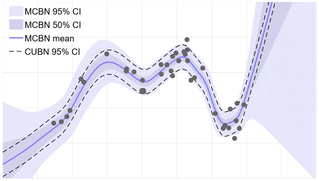
Figure 1: Illustration of the uncertainty obtained through batch normlization on a simple toy dataset.
As shown in Figure 2 from [], these approaches allow to represent uncertainty on predictions, potentially improving estimates on out-of-distribution examples. Recent work also argues that Bayesian approaches improve robustness against adversarial examples []. However, scaling these approaches to challenging datasets, e.g., in computer vision is still challenging.
- [] Alex Graves. Practical Variational Inference for Neural Networks. NIPS 2011: 2348-2356.
- [] Charles Blundell, Julien Cornebise, Koray Kavukcuoglu, Daan Wierstra. Weight Uncertainty in Neural Networks. CoRR abs/1505.05424 (2015).
- [] Max Welling, Yee Whye Teh. Bayesian Learning via Stochastic Gradient Langevin Dynamics. ICML 2011: 681-688.
- [] Nitish Srivastava, Geoffrey E. Hinton, Alex Krizhevsky, Ilya Sutskever, Ruslan Salakhutdinov. Dropout: a simple way to prevent neural networks from overfitting. J. Mach. Learn. Res. 15(1): 1929-1958 (2014).
- [] Sergey Ioffe, Christian Szegedy. Batch Normalization: Accelerating Deep Network Training by Reducing Internal Covariate Shift. ICML 2015: 448-456.
- [] Yarin Gal. Uncertainty in Deep Learning. PhD Thesis, University of Cambridge, 2016.
- [] Diederik P. Kingma, Max Welling. Auto-Encoding Variational Bayes. ICLR 2014.
- [] David M. Blei, Alp Kucukelbir, Jon D. McAuliffe. Variational Inference: A Review for Statisticians. CoRR abs/1601.00670 (2016).categorica
- [] C. J. Maddison, A. Mnih, and Y. W. Teh. The concrete distribution: A continuous relaxation of discrete random variables. CoRR, abs/1611.00712, 2016.
- [] Avrim Blum, Nika Haghtalab, Ariel D. Procaccia. Variational Dropout and the Local Reparameterization Trick. NIPS, 2015.
- [] Mattias Teye, Hossein Azizpour, Kevin Smith. Bayesian Uncertainty Estimation for Batch Normalized Deep Networks. ICML, 2018.
- [] Xuanqing Liu, Yao Li, Chongruo Wu, Cho-Jui Hsieh. Adv-BNN: Improved Adversarial Defense through Robust Bayesian Neural Network. ICLR (Poster) 2019.