Implementation of Felzenszwalb and Huttenlocher's Graph-Based Image Segmentation • David Stutz

Introduction

Felzenszwalb and Huttenlocher's [1] graph-based image segmentation algorithm is a standard tool in computer vision, both because of the simple algorithm and the easy-to-use and well-programmed implementation provided by Felzenszwalb. Recently, the algorithm has frequently been used as pre-processing tool to generate oversegmentations or so-called superpixels ‐ groups of pixels perceptually belonging together. In this line of work, the algorithm is frequently used as baseline for state-of-the-art superpixel algorithms.

The algorithm has also been extended to video [2]. In the course of my studies, I developed an implementation of the algorithm for video segmentation, as can be found on GitHub. As side product, the implementation can easily be adapted for image segmentation. The code is also available on GitHub:

Implementation on GitHub

Compared to the original implementation, the presented implementation tries to improve connectivity of the generated segments/superpixels. The underlying reasoning is that connectivity is an essential requirement of superpixel algorithms and has significant influence on evaluation metrics.

Algorithm

The algorithm is briefly described below (click to collpse):

P. F. Felzenswalb and D. P. Huttenlocher. Efficient graph-based image segmentation. International Journal of Computer Vision, volume 59, number 2, 2004.

After introducing SEEDS [1] and SLIC [2], this article focusses on another approach to superpixel segmentation proposed by Felzenswalb & Huttenlocher. The procedure is summarized in algorithm 1 and based on the following definitions. Given an image $I$, $G = (V, E)$ is the graph with nodes corresponding to pixels, and edges between adjacent pixels. Each edge $(n,m) \in E$ is assigned a weight $w_{n,m} = \|I(n) - I(m)\|_2$. Then, for subsets $A,B \subseteq V$ we define $MST(A)$ to be the minimum spanning tree of $A$ and

$Int(A) = max_{n,m \in MST(A)} \{w_{n,m}\}$,

$MInt(A,B) = min\{Int(A) + \frac{\tau}{|A|}, Int(B) + \frac{\tau}{|B|}\}$.

where $\tau$ is a threshold parameter and $MInt(A,B)$ is called the minimum internal difference between components $A$ and $B$. Starting from an initial superpixel segmentation where each pixel forms its own superpixel the algorithm processes all edges in order of increasing edge weight. Whenever an edge connects two different superpixels, these are merged if the edge weight is small compared to the minimum internal difference.

function fh(
        $G = (V,E)$ // Undirected, weighted graph.
    )
    sort $E$ by increasing edge weight
    let $S$ be the initial superpixel segmentation
    for $k = 1,\ldots,|E|$
        let $(n,m)$ be the $k^{\text{th}}$ edge
            if the edge connects different superpixels $S_i,S_j \in S$
                if $w_{n,m}$ is sufficiently small compared to $MInt(S_i,S_j)$
                    merge superpixels $S_i$ and $S_j$
    return $S$

Algorithm 1: The superpixel algorithm proposed by Felzenswalb & Huttenlocher.

The original implementation can be found on Felzenswalb's website. Generated superpixel segmentations can be found in figure 1.

Figure 1: Images from the Berkeley Segmentation Dataset [3] oversegmented using the algorithm proposed by Felzenswalb & Huttenlocher.

[1] R. Achanta, A. Shaji, K. Smith, A. Lucchi, P. Fua, S. Süsstrunk. SLIC superpixels. Technical report, École Polytechnique Fédérale de Lausanne, 2010.
[2] M. van den Bergh, X. Boix, G. Roig, B. de Capitani, L. van Gool. SEEDS: Superpixels extracted via energy-driven sampling. European Conference on Computer Vision, pages 13–26, 2012.
[3] P. Arbeláez, M. Maire, C. Fowlkes, J. Malik. Contour detection and hierarchical image segmentation. Transactions on Pattern Analysis and Machine Intelligence, volume 33, number 5, pages 898–916, 2011.

Implementation

The provided implementation can easily be installed using CMake. On Ubuntu, this might look as follows:

$ git clone https://github.com/davidstutz/graph-based-image-segmentation.git
$ cd graph-based-image-segmentation
$ mkdir build
$ cd build
$ cmake ..
$ make

The implementation then provided an easy-to-use command line tool to run the algorithm on a folder containing one or several images:

$ ../bin/cli --help
Allowed options:
  -h [ --help ]            produce help message
  --input arg              folder containing the images to process
  --threshold arg (=20)    constant for threshold function
  --minimum-size arg (=10) minimum component size
  --output arg (=output)   save segmentation as CSV file and contour images

A closer look at cli/main.cpp also demonstrates the usage of the algorithm from C++:

// Read the image to oversegment.
cv::Mat image = cv::imread(image_path);

// Segmentation is governed by the following two components, which can easily be extended
// as can be seen in `lib/graph_segmentation.h`:
// - GraphSegmentationEuclideanRGB defines the distance to use to compute the weights
// between pixels to be a Euclidean distance on RGB;
// - GraphSegmentationMagicThreshold defines how to decide whether ot segments/pixels
// should be merged, in the original case this is done based on the computed weights,
// see the paper or the description above.
GraphSegmentationMagicThreshold magic(threshold);
GraphSegmentationEuclideanRGB distance;

GraphSegmentation segmenter;
segmenter.setMagic(&magic);
segmenter.setDistance(&distance);

segmenter.buildGraph(image);
segmenter.oversegmentGraph();
// Enforce a specific minimum semgent size as also done by the original
// implementation.
segmenter.enforceMinimumSegmentSize(minimum_segment_size);

// The labels are stored in a matrix containing integer values
// referring to the segment id.
cv::Mat labels = segmenter.deriveLabels();

Results

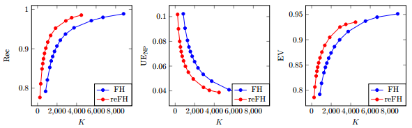
As comparison, both implementations ‐ the original one and the presented one ‐ are compared based on the following metrics. To this end, let $G = \{G_i\}$ be a ground truth segmentation where each segment $G_i$ refers to a set of pixels in the image. Further, let $S = \{S_j\}$ be a superpixel segmentation. Both segmentations are assumed to be partitions of the pixels contained in the image.

Boundary Recall [3] quantifies the fraction of boundary pixels in $G$ correctly captured by $S$. Let $F(G,S)$ and $TP(G,S)$ be the number of false negatives and true positive boundary pixels. Then Boundary Recall is defined by

$Rec(G, S) = \frac{TP(G,S)}{TP(G,S) + FN(G,S)}$

Higher Boundary Recall refers to better boundary adherence and, thus, better performance.

Undersegmentation Error measures the "leakage" of superpixels with respect to $G$ and, therefore, implicitly measures boundary adherence. The formulation by Neubert and Protzel [4] can be written as:

$UE(G,S) = \frac{1}{N}\sum_{G_i} \sum_{S_j \cap G_i \neq \emptyset} \min\{|S_j \cap G_i|,|S_j - G_i|\}$.

Lower Undersegmentation Error refers to better performance.

Explained Variation [5] quantifies the fraction of image variation captured by the superpixel segmentation:

$EV(S) = \frac{\sum_{S_j} |S_j|(\mu(S_j) - \mu(I))^2}{\sum_{x_n} (I(x_n) - \mu(I))^2}$

where $\mu(S_j)$ denotes the mean color of superpixel $S_j$, $\mu(I)$ denotes the mean color of the image, and $x_n$ denotes a pixel color.

Both algorithms provide exactly the same parameters and implement the algorithm as described in [1]. Therefore, both implementations were evaluated on the BSDS500 [3] using the same parameter settings. As the presented implementation tries to improve connectivity, it is likely to produce less superpixels for the same parameter settings. Figure 1 shows quantitative results with respect to the discussed metrics. Even though the presented implementation generates less superpixels, it demonstrates higher performance with respect to all three metrics.

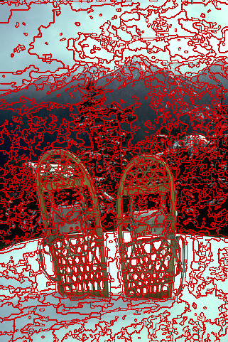
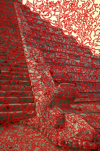
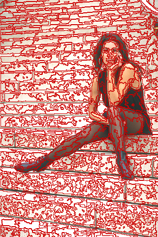
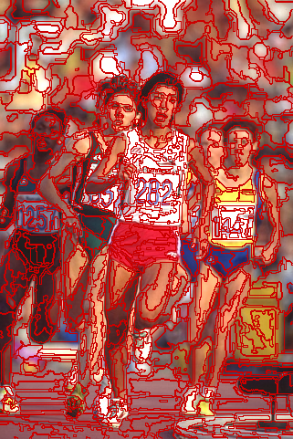
Figure 1 (click to enlarge): Quantitative results in terms of Boundary Recall $\text{Rec}$, Undersegmentation Error $\text{UE}$ and Explained Variation $\text{EV}$. Results have been computed on the test set of the BSDS500 using the same parameter settings. The results can also be downloaded as PDF.

Qualitative results are shown in Figure 2. Note the difference in the number of superpixels computed for the same parameters ‐ this illustrates the improved connectivity of the presented implementation. Also note that this difference is not necessarily perceivable, i.e. the number of superpixels counted for the original implementation may be higher due to small groups of pixels not being connected the the remaining pixels of the same superpixel. Except for this difference, the superpixels exhibit similar characteristics — or example the irregular boundaries within regions with mostly homogeneous color.

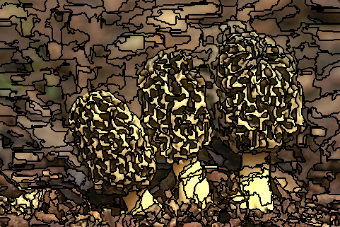
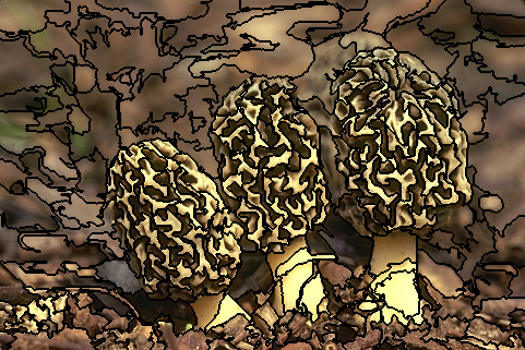
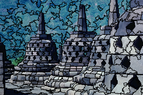
Figure 2 (click to enlarge): Qualitative results for both implementations on the BSDS500. Top row: results form the presented implementation with an average of $700$ superpixels over the three shown images. Middle row: results form the original implementation with a average of $800$ superpixels over the three shown images. Bottom row: results from the presented implementation using the same parameters as in the middle row, resulting in roughly $300$ superpixels over the three shown images. Note how the same parameters result in less superpixels in the presented implementation. This demonstrates improved connectivity. Also note that, visually, the results in the middle row and bottom row look similar. This suggests that the high number of superpixels of the original implementation is mainly due to small groups of pixels not being connected to the remaining pixels of the superpixel.

References

[1] P. F. Felzenswalb, D. P. Huttenlocher. Efficient graph-based image segmentation. International Journal of Computer Vision 59 (2) (2004) 167–181.
[2] M. Grundmann, V. Kwatra, M. Han, I. Essa. Efficient Hierarchical Graph Based Video Segmentation. CVPR, 2010.
[3] P. Arbeláez, M. Maire, C. Fowlkes, J. Malik. Contour detection and hierarchical image segmentation. IEEE Transactions on Pattern Analysis and Machine Intelligence 33 (5), 2011.
[4] P. Neubert, P. Protzel. Superpixel benchmark and comparison. In: Forum Bildverarbeitung, 2012.
[5] A. P. Moore, S. J. D. Prince, J. Warrell, U. Mohammed, G. Jones. Superpixel lattices. IEEE Conference on Computer Vision and Pattern Recognition, 2008.

IAM

DAVIDSTUTZ

ARTICLE