RESEARCH
Superpixel Algorithms
The latest Superpixel Benchmark [] also includes revised implementations of the graph-based image segmentation algorithm by Felzenswalb and Huttenlocher [] — referred to as FH — and SEEDS []. Separately from the benchmark, the implementations are discussed here.
Overview
FH [] and SEEDS [] are two very popular and efficient superpixel algorithms — actually, FH is a general image segmentation algorithm that is commonly used to generate oversegmentations. As part of the Superpixel Benchmark presented in [], revised implementations of FH and SEEDS are used for comparison purposes. The presented implementations demonstrate improved connectivity which can also be linked to better performance with regard to common metrics such as Boundary Recall [] and Undersegmentation Error []. The revised implementation of SEEDS — reSEEDS — additionally reduces runtime, while the performance improvement of the revised implementation of FH — reFH — comes at the cost of increased runtime. This page discusses both the algorithm's background and implementation. Additionally, a qualitative and quantitative comparison is provided.
Related Implementations
Regarding SEEDS, available implementations include the original implementation and the OpenCV implementation. Considering FH, the original implementation can be found here.
Download and Citing
The implementations are available on GitHub:
reSEEDSreFHIf you use these implementations, consider citing the corresponding benchmark:
@article{StutzHermansLeibe:2016,
    author    = {David Stutz and Alexander Hermans and Bastian Leibe},
    title     = {Superpixels: An Evaluation of the State-of-the-Art},
    journal   = {CoRR},
    volume    = {abs/1612.01601},
    year      = {2016},
    url       = {https://arxiv.org/abs/1612.01601},
}
reSEEDS was originally implemented as part of the following thesis:
@misc{Stutz:2014,
    author = {David Stutz},
    title = {Superpixel Segmentation using Depth Information},
    month = {September},
    year = {2014},
    institution = {RWTH Aachen University},
    address = {Aachen, Germany},
    howpublished = {http://davidstutz.de/},
}
SEEDS Revised (reSEEDS)
Given an image $I: \{1, \ldots, W\} \times \{1, \ldots, H\} \rightarrow \{0, \ldots, 255\}^3$, the algorithm starts by grouping pixels into blocks of size $w^{(1)} \times h^{(1)}$. These blocks are then further arranged into blocks of $2 \times 2$. This scheme is applied recursively to form a hierarchy of blocks such that blocks at level $l$ have size
$w^{(l)} = w^{(1)} \cdot 2^{l-1}$ and $h^{(l)} = h^{(1)} \cdot 2^{l-1}$.
This is repeated for a total of $L$ levels. Therefore, the number of superpixels is calculated as follows:
$S = \frac{W}{w^{(L)}} \cdot \frac{H}{h^{(L)}}$
where we assume the divisions to be integer divisions. In practice, this means that the number of levels $L$ and the initial block size $w^{(1)} \times h^{(1)}$ need to be dervied from the desired number of superpixels $K$.
The initial superpixel segmentation is refined by exchanging blocks of pixels as well as single pixels between neighboring superpixels. Therefore, let $B_i^{(l)} \subseteq \{1,\ldots, W\}\times\{1,\ldots, H\}$ be a block of pixels at level $l$ and $S_j$ be a superpixel. With $h_{B_i^{(l)}}$ we denote the color histogram of block $B_i^{(l)}$. Then, the similarity of block $B_i^{(l)}$ and superpixel $S_j$ is given by the intersection of the corresponding histograms:
$\cap(h_{B_i^{(l)}}, h_{S_j}) = \sum_{q = 1}^Q \min\{h_{B_i^{(l)}}(q), h_{S_j}(q)\}$
where we assume the histograms to be normalized. Furthermore, the similarity of a single pixel $x_n$ and the superpixel $S_j$ is given by
$h_{S_j}(h(x_n))$
where $h(x_n)$ is the histogram bin of pixel $x_n$. Given this basic framework, Algorithm 1 describes a simple implementation of SEEDS.
function SEEDS(
        $I$, // Color image.
        $w^{(1)} \times h^{(1)}$, // Initial block size.
        $L$, // Number of levels.
        $Q$ // Histogram size.
    )
    initialize the block hierarchy and the initial superpixel segmentation
    // Initialize histograms for all blocks and superpixels:
    for $l = 1$ to $L$
        // At level $l = L$ these are the initial superpixels:
        for each block $B_i^{(l)}$
            initialize histogram $h_{B_i^{(l)}}$
    // Block updates:
    for $l = L - 1$ to $1$
        for each block $B_i^{(l)}$
            let $S_j$ be the superpixel $B_i^{(l)}$ belongs to
            if a neighboring block belongs to a different superpixel $S_k$
                if $\cap(h_{B_i^{(l)}}, h_{S_k}) > \cap(h_{B_i^{(l)}}, h_{S_j})$
                    $S_k := S_k \cup B_i^{(l)}$, $S_j := S_j - B_i^{(l)}$
    // Pixel updates:
    for $n = 1$ to $W\cdot H$
        let $S_j$ be the superpixel $x_n$ belongs to
        if a neighboring pixel belongs to a different superpixel $S_k$
            if $h_{S_k}(h(x_n)) > h_{S_j}(h(x_n))$
                $S_k := S_k \cup \{x_n\}$, $S_j := S_j - \{x_n\}$
    return $S$
As alternative, the similarity of a pixel $x_n$ and a superpixel $S_j$ can be expressed as distance:
$d(x_n, S_j) = \|I(x_n) - I(S_j)\|_2$
where $I(S_j)$ is the mean color of the superpixel $S_j$. This variant of pixel updates is called mean pixel updates.
Compactness and Smoothness
[] discuss both a compactness and a smoothness term. The former is comparably easy to implement — adapting the distance used for mean pixel updates as follows:
$d(x_n, S_j) = \|I(x_n) - I(S_j)\|_2 + \lambda\|x_n - \mu(S_j)\|_2$
where $\mu(S_j)$ is the center position of superpixel $S_j$.
The latter tries to encourage smooth superpixel boundaries. For each pair of pixels $(x_n, x_m)$ belonging to different superpixels, a $3 \times 4$ or $4\times 3$ neighborhood is considered. Then, the number $N_{n,m,j}$ of pixels belonging to superpixel $S_j$ as well as the number $N_{n,m,k}$ of pixels belonging to superpixel $S_k$ is counted. Then, the histogram-based criterion for pixel updates is weighted by these counts. However, the smoothness term is not implemented for mean pixel updates.While the compactness term is discussed in [], neither the OpenCV implementation nor the original implementation implement the compactness term (at the time of writing).
Implementation
The implementation was done with ease-to-use and efficiency in mind. It also easily integrates with OpenCV. In the following, we provide building and usage instructions. More details can be found in the GitHub repository.
The implementation was previously discussed in this article: Efficient High-Quality Superpixels: SEEDS Revised.
Building
The following steps assume a working OpenCV installation (that is accessible through CMake's find_package) and are based on an Ubuntu operating system:
$ sudo apt-get install build-essential cmake libboost-dev-all
$ git clone https://github.com/davidstutz/seeds-revised.git
$ cd seeds-revised/build
$ cmake ..
$ make
Usage
SeedsRevised.h provides two classes: SEEDSRevised implements the original SEEDS algorithm including smoothness term; SEEDSRevisedMeanPixels implements the variant with mean pixel updates and compactness term. Usage is comparably simply given an OpenCV image and a desired number of superpixels:
cv::Mat image = cv::imread(filepath);
int superpixels = 800;
int iterations = 2;

SEEDSRevisedMeanPixels seeds(image, superpixels);
seeds.initialize();
seeds.iterate(iterations);

// Retrieve labels and put out contour image.
int** labels = seeds.getLabels();
SEEDSRevisedMeanPixels provides the following parameters (SEEDSRevised provides a subset):
- image: the image in the form of a cv::Mat in BGR color space.
- desiredNumberOfSuperpixels: number of desired superpixels.
- numberOfBins: number of bins per channel used to calculate the color histograms (see above).
- neighborhoodSize: size of the smoothing window as explained above; $1$ is usually sufficient, greater values will slow down the algorithm and result in smoother superpixels.
- minimumConfidence: minimum difference of histogram intersection required for block updates.
- spatialWeight: only available for
SEEDSRevisedMeanPixels; used to weight the compactness term. - colorSpace: the color space to use, one of
SEEDSRevised::BGR,SEEDSRevised::LAB,SEEDSRevised::HSV,SEEDSRevised::LUV,SEEDSRevised::XYZorSEEDSRevised::YCRCB.
A complete usage example can be found in cli/main.cpp.
FH Revised (reFH)
Given an image $I$, $G = (V, E)$ is the graph with nodes corresponding to pixels, and edges between adjacent pixels. Each edge $(n,m) \in E$ is assigned a weight $w_{n,m} = \|I(x_n) - I(x_m)\|_2$. Then, for superpixels $S_i,S_j \subseteq V$ we define $MSTS_i)$ to be the minimum spanning tree of $S_i$ and
$Int(S_i) = max_{n,m \in MST(S_i)} \{w_{n,m}\}$,
$MInt(S_i,S_j) = min\{Int(S_i) + \frac{\tau}{|S_i|}, Int(S_j) + \frac{\tau}{|S_j|}\}$.
where $\tau$ is a threshold parameter and $MInt(S_i,S_j)$ is called the minimum internal difference between superpixels $S_i$ and $S_j$. Starting from an initial superpixel segmentation where each pixel forms its own superpixel the algorithm processes all edges in order of increasing edge weight. Whenever an edge connects two different superpixels, these are merged if the edge weight is small compared to the minimum internal difference.
function FH(
        $G = (V,E)$ // Undirected, weighted graph.
    )
    sort $E$ by increasing edge weight
    let $S$ be the initial superpixel segmentation
    for $k = 1,\ldots,|E|$
        let $(n,m)$ be the $k^{\text{th}}$ edge
            if the edge connects different superpixels $S_i,S_j \in S$
                if $w_{n,m}$ is sufficiently small compared to $MInt(S_i,S_j)$
                    merge superpixels $S_i$ and $S_j$
    return $S$
Algorithm 2: The superpixel algorithm proposed by Felzenswalb & Huttenlocher.
Implementation
reFH was originally meant as an experimental prototype. Thus, the algorithm is flexible in which distance is used to compute the edge weights and allows to easily implement custom distances as well as threshold mechanisms. The implementation interfaces to OpenCV.
The implementation was previously discussed in this article: Implementation of Felzenszwalb and Huttenlocher’s Graph-Based Image Segmentation.
Building
The following steps assume a working OpenCV installation (that is accessible through CMake's find_package) and are based on an Ubuntu operating system:
$ git clone https://github.com/davidstutz/graph-based-image-segmentation.git
$ cd graph-based-image-segmentation
$ mkdir build
$ cd build
$ cmake ..
$ make
Usage
graph_segmentation.h provides the main class, GraphSegmentation, which can be used as follows:
cv::Mat image = cv::imread(filepath);

GraphSegmentationMagicThreshold magic(threshold);
GraphSegmentationManhattenRGB distance;

GraphSegmentation segmenter;
segmenter.setMagic(&magic);
segmenter.setDistance(&distance);

segmenter.buildGraph(image);
segmenter.oversegmentGraph();
segmenter.enforceMinimumSegmentSize(minimum_segment_size);

cv::Mat labels = segmenter.deriveLabels();
GraphSegmentation has two components:
- the used distance, set via
setDistance, defining the distance used to compute the edge weights; - and the used threshold mechanism — called "magic" —, set via
setMagic, that defines when two superpixels are merged.
Per default, the latter corresponds to the criterion described in Algorithm 2; however, this criterion can easily be adapted. The default distance used is the Manhatten RGB distance.>/p>
A complete usage example can be found in cli/main.cpp.
Results
As subsumed in the latest Superpixel Benchmark, qualitative and quantitative results are presented. We compare the original implementations with the presented implementations. The parameters for all algorithms were optimized separately on the validation set of the BSDS500 dataset [] as described in []. Used metrics are discussed first.
Metrics
Boundary Recall [3] quantifies the fraction of boundary pixels in $G$ correctly captured by $S$. Let $F(G,S)$ and $TP(G,S)$ be the number of false negatives and true positive boundary pixels. Then Boundary Recall is defined by$Rec(G, S) = \frac{TP(G,S)}{TP(G,S) + FN(G,S)}$
Higher Boundary Recall refers to better boundary adherence and, thus, better performance.
Undersegmentation Error measures the "leakage" of superpixels with respect to $G$ and, therefore, implicitly measures boundary adherence. The formulation by Neubert and Protzel [4] can be written as:
$UE(G,S) = \frac{1}{N}\sum_{G_i} \sum_{S_j \cap G_i \neq \emptyset} \min\{|S_j \cap G_i|,|S_j - G_i|\}$.
Lower Undersegmentation Error refers to better performance.
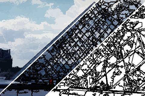
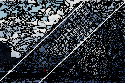
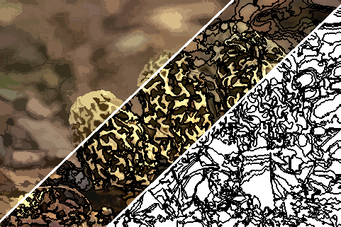
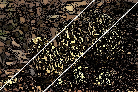
Qualitative


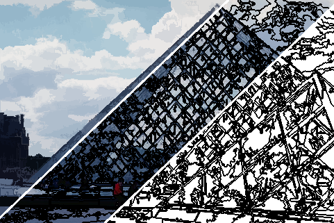
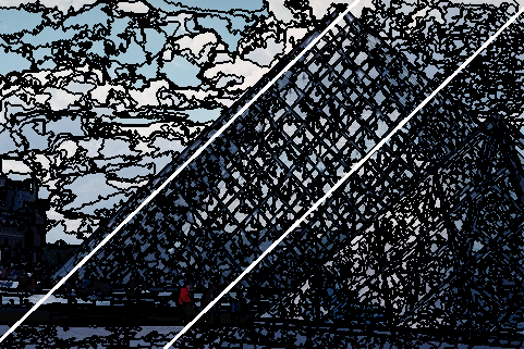
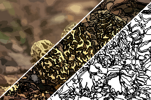
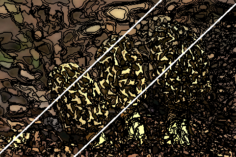

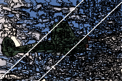


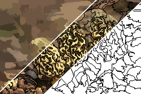

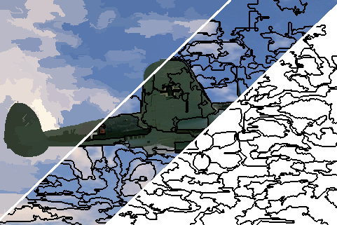
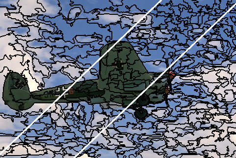

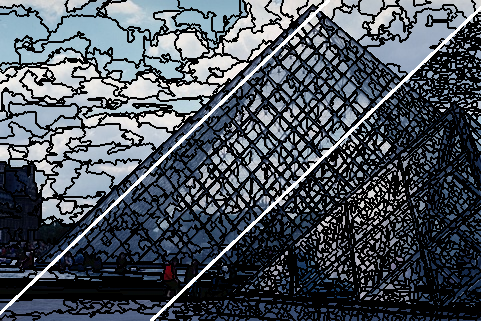
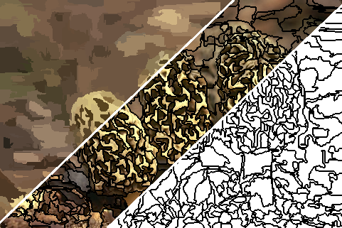

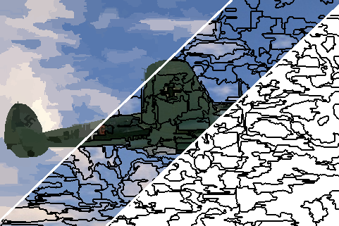
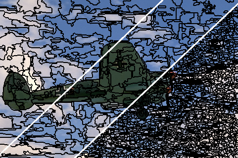
Quantitative
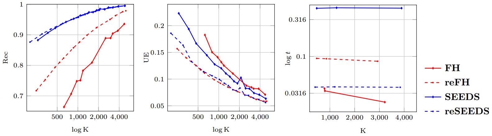
Figure 1 shows Boundary Recall (Rec), Undersegmentation Error (UE) and runtime (t) plotted against the number of generated superpixels for all four evaluated implementations, SEEDS, reSEEDS, FH and reFH. As can be seen, reFH clearly outperforms FH with respect to Rec and UE, however, the increased performance comes at the cost of increased runtime. SEEDS, in contrast, demonstrates very high Rec such that reSEEDS is not able to outperform reSEEDS significantly. Regarding UE, reSEEDS is able to outperform SEEDS. However, the difference is not as significant as in the cases of FH and reFH. Finally, reSEEDS runs significantly faster than SEEDS. Here, we note that SEEDS represents the original implementation — the OpenCV implementation of SEEDS is significantly more efficient that#n the original one. However, we do not have experimental results comparing reSEEDS to the OpenCV implementation.
Conclusion
We presented two revised implementations, reSEEDS and reFH, of popular superpixel algorithms, namely SEEDS [] and FH []. Overall, our revised implementations illustrate that revisiting the original implementations of superpixel algorithms might be beneficial to increase performance and reduce runtime. Note that similar experiments are discussed in [] in more detail.
Acknowledgements
See acknowledgements here and here.
References
- [] D. Stutz, A. Hermans, B. Leibe. Superpixels: An Evaluation of the State-of-the-Art. CoRR abs/1612.01601, 2016.
- [] M. van den Bergh, X. Boix, G. Roig, B. de Capitani, L. van Gool. SEEDS: Superpixels extracted via energy-driven sampling. ECCV, 2012.
- [] M. Van den Bergh, X. Boix, G. Roig, L. J. Van Gool. SEEDS: Superpixels Extracted via Energy-Driven Sampling. CoRR abs/1309.3848, 2013.
- [] P. F. Felzenswalb, D. P. Huttenlocher. Efficient graph-based image segmentation. IJCV, 2004.
- [] P. Arbel´aez, M. Maire, C. Fowlkes, J. Malik. Contour detection and hierarchical image segmentation. PAMI, 2011.
- [] P. Neubert, P. Protzel. Superpixel benchmark and comparison. Forum Bildverarbeitung, 2012.