As part of my master thesis, I started working on 3D convolutional neural networks — particularly for 3D object recognition and shape completion. In the literature, learning on 3D data is an exciting topic as researchers are still trying to figure out the proper data representation for different modalities and how to train deep models efficiently on these representations. In this article, I want to discuss several relevant papers in this research area.
Overview
One of the standard benchmarks for 3D convolutional neural networks is the ModelNet dataset []. It consists of 10 (or 40) different categories of objects (such as sofa, chair, table, monitor etc.). For each category several hundred CAD models are provided and the task is to classify these CAD models. In addition, the dataset as also commonly used for for related tasks such as shape completion or generative shape modeling. Of course, convolutional neural networks can easily be trained on 3D voxel grids (e.g. occupancy grids) of these CAD models. However, are occupancy grids the best data representations? How can the network be trained efficiently? And what should the architecture look like? These questions (and more) are key to most of the publications in this research area.
3D data may take different forms. For example, videos can be seen as 3D data (where the third dimension represents time). In contrast, for many medical imaging tasks as well as for CAD models or point clouds (e.g. from LiDAR sensors) the third dimension represents depth. Often, the data is additionally very sparse. 3D convolutional neural networks are applicable in all these cases. For example, in [] for action recognition in videos, in [] for microbleed detection in MR volumes, in [] for object recognition on point clouds and in [][][][][][][][] — among others — for object recognition on voxel grids. Additionally, it is not yet clear whether volumetric representations are better at all. Some works [][] also use so-called multi-view convolutional neural networks. These are regular, 2D convolutional neural networks applied on several different views of the object.
In addition to the problem of data representation, efficient training is problematic. Recent publications usually work on small voxel grids in the order of $32^3$ or $64^3$. Different publications, among others [][][][], are discussing approaches to reduce the computational complexity of convolutional neural networks to allow higher resolution and/or efficient training. Similar to multi-view convolutional neural networks, other works [][] propose specific layer types to reduce 3D (voxel) grids to 2D (pixel) grids.
Reading Notes
The ModelNet benchmark:
Wu et al. present 3D ShapeNets - based on convolutional deep belief networks, they tackle the problem of shape recognition and retrieval. They also introduce the ModelNet dataset consisting of roughly 150k CAD models of 660 categories. For evaluation, however, they use 10-category or 40-category subset (this is also used in several related publications [1,2]). Examples are shown in Figure 1.
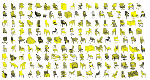
Figure 1 (click to enlarge): 3d shape models included in the ModelNet dataset include various categories such as window, aircraft, shelf, truck, fence, coffee table etc.
The used deep belief net architecture is summarized in Figure 2 and consists primarily of 3 convolutional layers. While background on deep belief nets can for example be found in [3], the energy of a convolutional layer is given by
$E(v,h) = -\sum_f \sum_j (h_j^f(W^f \star v)_j + c^fh_j^f) - \sum_l b_l v_l$
where $v_l$ refer to the visible units, $h_j^f$ refer to the hidden units in a given feature channel $f$ and $W^f$ is the convolution kernel for channel $f$. They also include a stride in the convolutional layer, see Figure 2.
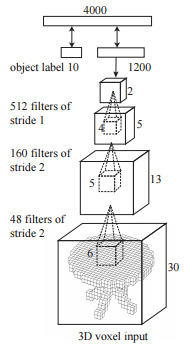
Figure 2 (click to enlarge): Illustration of the used deep belief network. Three convolutional layer are followed by two fully connected layers. The number and size of the used kernels is included. The model is trained on $24 \times 24 \times 24$ models which are padded up to $30 \times 30 \times 30$.
The training procedure is split in pre-training and fine-tuning. For pre-training, the three convolutional layers and the fully connected layers are trained using contrastive divergence. For the top layer, fast persistent contrastive divergence is used. The procedure proceeds layer by layer, i.e. as soon as the weights in the lower level are trained, they are fixed and the next layer is trained. Fine-tuning is based on a wake-sleep similar algorithm.
They discuss two applications in detail, 3d reconstruction from 2.5d (i.e. RGBD images) and next-best-view prediction. In the later problem, given a single view point, the task is to predict the best next view in order to reduce uncertainty regarding the category. For the former problem, a voxel cloud is constructed from the given RGBD image. All unobserved voxels (i.e. lying behind the observed surface) are treated as missing information. To recover both the missing voxels and the category, Gibbs sampling is used to approximate the posterior $p(y|x_o)$ where $y$ is the category and the input $x$ is splitted in observed voxels $x_o$ and unobserved voxels $x_u$. Initially setting $x_u$ to random values, these are propagated up to sample the category $y$. The sampled high-level signal is propagated down to sample the unobserved voxels $x_u$. This process is repeated up to $50$ times. Results are shown in Figure 3.

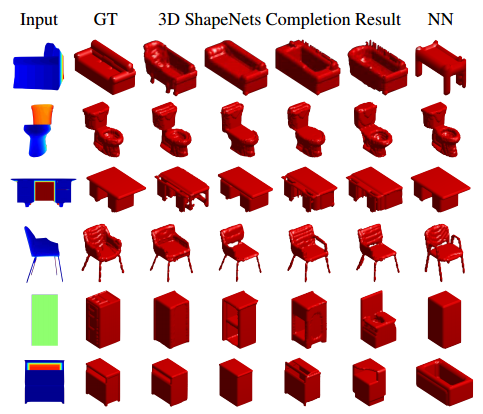
Figure 3 (click to enlarge): Examples of shape generation for some categories (left); examples of shape completion (right).
- [1] Yangyan Li, Sören Pirk, Hao Su, Charles Ruizhongtai Qi, Leonidas J. Guibas. FPNN: Field Probing Neural Networks for 3D Data. CoRR, abs/1605.06240.
- [2] Charles Ruizhongtai Qi. Hao Su, Matthias Nießner, Angela Dai, Mengyuan Yan, Leonidas Guibas. Volumetric and Multi-View CNNs for Object Classification on 3D Data. CVPR, 2016.
- [3] Ian Goodfellow, Yoshua Bengio, Aaron Courville. Deep Learning. MIT Press, 2016.
Some approaches to 3D object recognition, usually evaluated on ModelNet:
Hegde and Zadeh discuss the fusion of multi-view convolutional neural networks (CNNs) and volumetric/3D CNNs for shape classification on ModelNet []. They combine a multi-view CNN similar to [] but based on AlexNet with two volumetric CNNs – the architectures are shown in Figure 1 and Figure 2 respectively. Both architectures are quite simple and small, adding only few parameters to the multi-view CNN. Interestingly, the used convolutional kernels have size $3 \times 3 \times 30$ for volumes of size $30^3$. This way, they hope to learn long-range correlation of the voxels assuming that the models are trained on all possible orientations of the shapes.
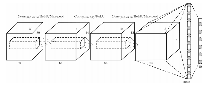
Figure 1 (click to enlarge): Illustration of the architecture of their “first” volumetric CNN.
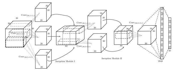
Figure 2 (click to enlarge): The network architecture of their “second” volumetric CNN. The architecture lends ideas from the Inception modules discussed for GoogLeNet [].
Experimental results show that, used alone, the multi-view CNN is still superior to the volumetric CNNs. But on the other hand, these are trained and evaluated on a resolution of $30^3$ only. When combining two volumetric CNNs with their multi-view CNN they are able to outperform the state-of-the-art on ModelNet. They combine the models using a linear combination of the class scores where the weights are determined using cross-validation.
- [] Z. Wu, S. Song, A. Khosla, F. Yu, L. Zhang, X. Tang, and J. Xiao. 3d shapenets: A deep representation for volumetric shapes. CVPR, 2015.
- [] H. Su, S. Maji, E. Kalogerakis, and E. Learned-Miller. Multiview convolutional neural networks for 3d shape recognition. CVPR, 2015.
- [] C. Szegedy, W. Liu, Y. Jia, P. Sermanet, S. E. Reed, D. Anguelov, D. Erhan, V. Vanhoucke, and A. Rabinovich. Going deeper with convolutions. CoRR, 2014.
Girdhar et al. present the so-called TL-embedding network, a combination of a 3D auto-encoder to reconstruct voxel grid and a AlexNet-like [] network to infer the voxel grid from 2D images. Their main motivation is two address two questions:
- How to learn a generative representation in 3D?
- Can this representation be predicted from 2D?
The proposed architecture is depicted in Figure 1 and consists of a 3D auto-encoder learning a $64$-dimensional representation. The auto-encoder consists of several convolutional and deconvolutional layers, the details can be found in the figure. Although not explicitly discussed, they predict occupancy grid and measure error using a voxel-wise cross-entropy loss. For prediction from 2D, they use a AlexNet-like architecture (using the pre-trained weights), taking an image as input and predicting the 64-dimensional representation learned by the auto-encoder.

Figure 1 (click to enlarge): Illustration of the network architecture. During training (T-Network) an auto-encoder and a AlexNet-like ConvNet are trained jointly. During testing (L-Network), the representations predicted by the AlexNet are fed into the decoder of the auto-encoder to predict a voxel grid.
For training, they generate data from CAD models by rendering them in front of random background taken from the internet. Training is done in three stages. First, the auto-encoder is trained separately. Then, the AlexNet is trained to regress the learned $64$-dimensional representation (while keeping the auto-encoder fixed). Finally, both models are fine-tuned jointly.
They provide several qualitative and quantitative experimental results. Reconstruction results using the auto-encoder are shown in Figure 2, compared to a PCA baseline. Regarding the first question, they conduct experiments regarding the smoothness and interpretability of the learned representations. Figure 3 shows examples where two representations are interpolated and Figure 5 showsn examples of adapting individual dimensions. They also provide experiments regarding shape retrieval from images, see the paper for details.
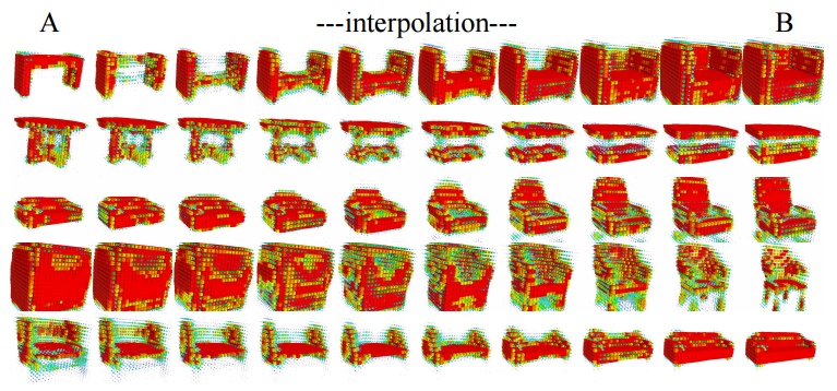
Figure 2 (click to enlarge): Shape interpolation by interpolating between two fixed representations and using the decoder to predict a voxel grid.
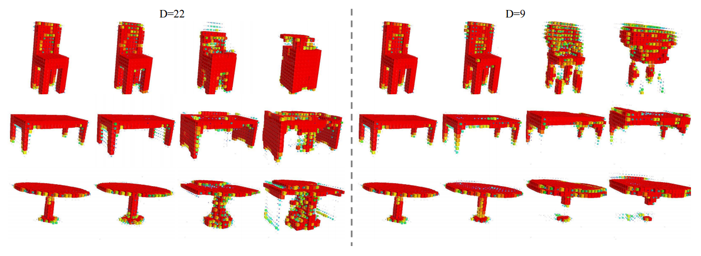
Figure 3 (click to enlarge): Illustration of adapting individual dimensions in the learned representation.
- [] Krizhevsky, A., Sutskever, I., Hinton, G.E.: Imagenet classification with deep convolutional neural networks. In: NIPS. pp. 1097–1105 (2012).
Sharma et al. use a volumetric convolutional denoising auto-encoder for shape completion and classification on the ModelNet [] Dataset. Their approach is comparably simple — the extension of the regular denoising auto-encoder to volumetric data is straight forwards on the used resolution of $30^3$. The architecture is quite simple and illustrated in Figure 1. A dropout layer after the input simulates noise and a bottleneck layer of dimensionality $6912$ is used.

Figure 1 (click to enlarge): The volumetric, convolutional denoising auto-encoder architecture used by Sharma et al.
In experiments on the ModelNet [] Dataset, they demonstrate the applicability of their model for classification and shape completion. For classification they outperform the ShapeNet model [] both when training an SVM on the $6912$ dimensional representation and when fine-tuning by adding two additional fully connected layers. However, VoxNet [] still outperforms their approach. Qualitative results for shape completion on random noise and slicing noise are shown in Figure 2 and 3, respectively. It seems as if the model struggles most with the low resolution. Especially for slicing noise, the model performs poorly because of the low resolution.
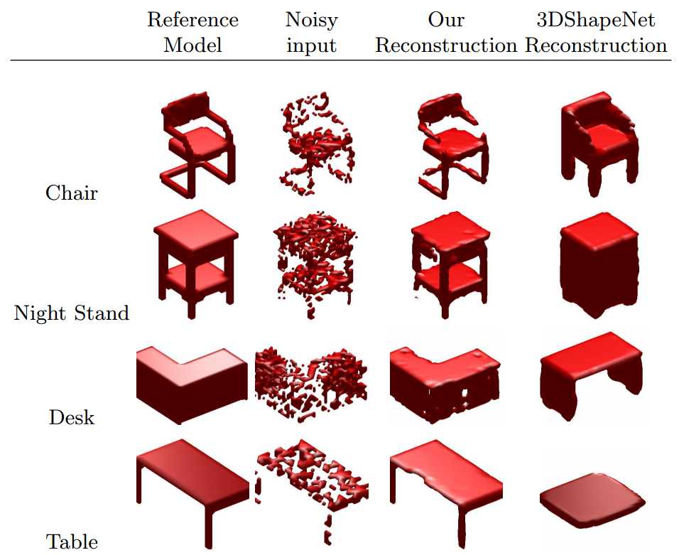
Figure 2 (click to enlarge): Qualitative results for shape completion from random noise. Comparison to ShapeNet [].
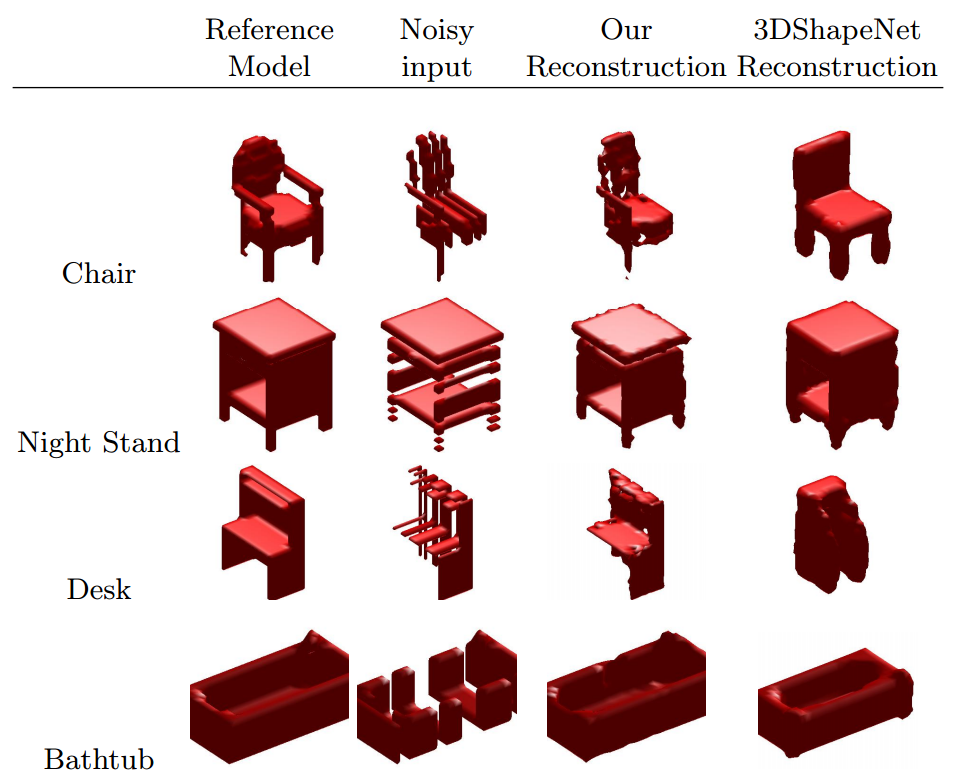
Figure 3 (click to enlarge): Qualitative results of shape completion on slicing noise and comparison to ShapeNet [].
- [] Wu, Z., Song, S., Khosla, A., Yu, F., Zhang, L., Tang, X., Xiao, J.: 3d shapenets: A deep representation for volumetric shapes. In: CVPR. (2015).
- [] Su, H., Maji, S., Kalogerakis, E., Learned-Miller, E.G.: Multi-view convolutional neural networks for 3d shape recognition. In: Proc. ICCV. (2015).
Brock et al. discuss voxel-based variational auto-encoders for shape reconstruction as well as deep 3D convolutional neural networks for shape classification. Regarding shape reconstruction, the variational auto-encoder architecture is illustrated in Figure 1 including the corresponding filter sizes. They make use of exponential linear units [1] and Xavier initialization [2]. Instead of pooling, they use strided convolution for downsampling and fractionally strided convolution [3] for upsampling. The loss function is augmented to better fit the task of reconstructing very sparse 3D occupancy grids. To this end, they augment the binary cross entropy per pixel to weight false positives and false negatives differently:
$\mathcal{L} = - \gamma t \log(o) - (1 - \gamma)(1 - t) \log(1 - o)$
where $t$ is the target, $o$ the output and the weight $\gamma$ is set to $0.97$. Furthermore, the target $t$ is re-scaled to lie in $\{-1,2\}$ and the output is re-scaled to $[0.1,1)$. The intention is to avoid vanishing gradients during training. Still, these numbers look rather random — no theoretical or experimental validation is provided. The model is trained on augmented data including horizontal flips, random translations and noise. In experiments, they validate that the modified binary cross entropy aids training. Reconstruction and interpolation results are shown in Figure 2.
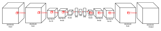
Figure 1 (click to enlarge): Architecture of the used variational auto-encoder for 3D shape reconstruction.

Figure 2 (click to enlarge): Reconstruction and interpolation results.
For 3D shape classification, Brock et al. use deep 3D convolutional networks combining many interesting techniques with the newly proposed Voxeption blocks. The overall architecture is shown in Figure 3 and discussed in the following. DS describes a Voxception Downsampling block as illustrated in Figure 4 (left). The idea is to let the network decide which downsampling approach is most useful for the task. Thus, the block concatenates downsampled versions of the input feature maps where downsampling is performed using max pooling, average pooling or different convolutional layers with stride. VRN describes a Voxception ResNet block, illustrated in Figure 4 (right). The intention is to give the network the possibility to choose between different convolutional layers, in this case $1 \times 1 \times 1$ vs. $3 \times 3 \times 3$. This approach is combined with the design of residual units [4]. In the spirit of [5], they drop the non-residual connections of the network with varying probability, see the paper for details. The overall network architecture consists of four blocks all containing a VRN and a DS block, followed by a final residual convolutional layer, a pooling layer and a fully connected layer.
For training, Brock et al. change the binary voxels to lie in $\{-1,5\}$ to encourage better training and adapt the learning rate manually based on the validation loss. The training set is augmented using random, horizontal flipping, translation and incorporating different rotations of each sample. The model is initialized on a training set augmented with 12 rotations and fine-tuned on 24 orientations per sample. For testing, they use a small ensemble, which significantly boosts performance and outperforms the compared state-of-the-art.
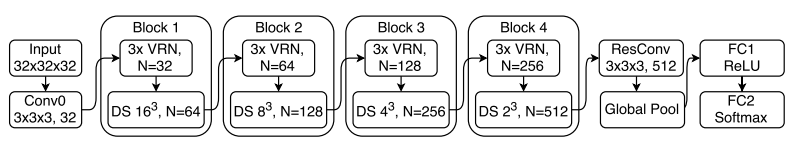
Figure 3 (click to enlarge): Illustration of the overall architecture used for 3D shape classification. The architecture mainly consists of 4 blocks comprising so-called Voxceptiom ResNet blocks (VRN) and Voxception Downsampling blocks (DS), see the text for details.

Figure 4: Illustration of the Voxception Downsampling (DS) block and the Voxception ResNet (VRN) block.
- [1] D.-A. Clevert, T. Unterthiner, S. Hochreiter. Fast and accurate deep network learning by exponential linear units (elus). ICLR, 2016.
- [2] X. Glorot, Y. Bengio. Understanding the difficulty of training deep feedforward neural networks. AISTATS, 2010.
- [3] V. Dumoulin, F. Visin. A guide to convolution arithmetic for deep learning. CoRR, 2016.
- [4] K. He, X. Zhang, S. Ren, J. Sun. Deep residual learning for image recognition. CVPR, 2016.
- [5] G. Huang, Y. Sun, Z. Liu, D. Sedra, K. Q. Weinberger. Deep networks with stochastic depth. CoRR, 2016.
Sedaghat et al. analyze the influence of orientation boosting, i.e. introducing orientation estimation as auxiliary task, for 3D shape and object recognition in VoxNets [1]. On several datasets including ModelNet [2] and KITTI [3], they introduce orientation estimation as auxiliary task in three different ways, as illustrated in Figure 1. The corresponding loss functions used are composites consisting of the individual cross-entropy loss functions.
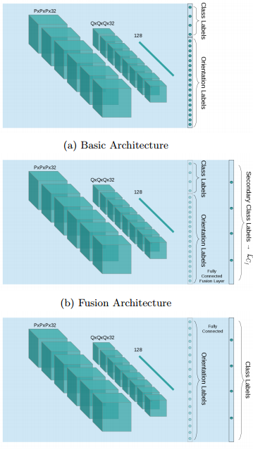
Figure 1 (click to enlarge): The three different approaches proposed to integrate orientation estimation into the original classification task. First, the orientations are binned and the created classes are appended to the original classes. Second, the original and orientation classes are interpreted as additional layer and the original classes are stacked on top. Third, The orientation classes are understood as additional layer and the original classes are supposed to be inferred form the orientation labels.
In experiments, they show improved classification accuracy when incorporating orientation estimation. However, the results do not specifically favor one of the proposed approaches but rather are spread seemingly random across the three architectures. Based on the results, Sedaghat et al. also introduce a visualization technique they call dominant signal paths. These paths are computed by backtracking the most significant units contributing to the predicted class. Through this new visualization, they show that their architectures become sensitive to orientation, in contrast to the original VoxNet.
Unfortunately, the presented attempts to incorporate orientation estimation are quite simple — i.e. the architecture is left un-modified and the orientation classes are always predicted at the top of the architecture. Still, the visualization technique has the potential to guide architecture design to incorporate orientation.
- [1] D. Maturana, S. Scherer. VoxNet: A 3D Convolutional Neural Network for Real-Time Object Recognition. IROS, 2015.
- [2] Z. Wu, S. Song, A. Khosla, F. Yu, L. Zhang, X. Tang, J. Xiao, J.. 3D ShapeNets: A Deep Representation for Volumetric Shapes. CVPR, 2015.
- [3] A. Geiger, P. Lenz, R. Urtasun. Are we ready for Autonomous Driving? The KITTI Vision Benchmark Suite. CVPR, 2012.
Wu et al. propose an extension to the VAE-GAN model [1] to 3D data in order to tackle 3D shape generation and classification. In the VAE-GAN model a variational autoencoder is combined with a generative adversarial network as illsutrated in Figure 1. For details, see [1].
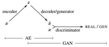
Figure 1 (click to enlarge): Illustration of the VAE-GAN model proposed by Larsen et al. [1] and generalized to 3D data by Wu et al. The variational auto-encoder consisting of encoder and decoder represents the connection between the input $x$ and the latent variables (or the code) $z$. The adversarial generative network combines a generator and a discriminator. The generator tries to generate data and fool the discriminator into believing that the generated data is real. In the VAE-GAN model, the decoder and the generator represent the same model, i.e. share their parameters. Training is performed by minimizing a combination of the losses of both models.
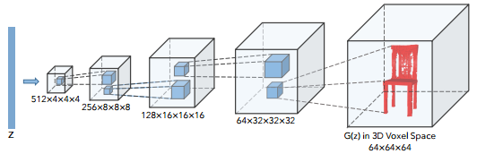
The network architecture used for the generator is illustrated in Figure 2. The discriminator mirrors this structure. The encoder is a convolutional neural network operating on images (not 3D data) consisting of 5 convolutional layers followed by batch normalization and ReLU activation layers. The idea is that the encoder allows to get the latent variables $z$ from a 2D image and then perform 3D reconstruction using the decoder/generator, taking $z$ as input, to generated a 3D shape.
Results of data generation are shown in Figure 3. For visualization, z is sampled form a uniform distribution and the largest connected component is visualized. 3D reconstruction results are demonstrated in Figure 4.
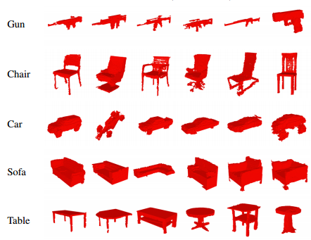
Figure 3 (click to enlarge): Generation results without a reference object.
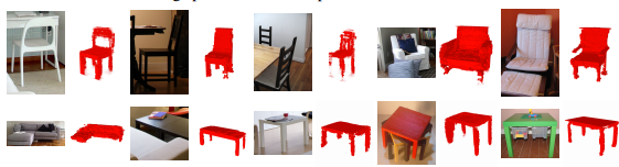
Figure 3 (click to enlarge): 3D reconstruction results.
- [1] Anders Boesen Lindbo Larsen, Søren Kaae Sønderby, Ole Winther. Autoencoding beyond pixels using a learned similarity metric. ICML, 2016.
Su et al., also motivated by the work from Wu et al. [1], proposes a simple convolutional neural network architecture to fuse information from different views to tackle 3D shape recognition. Their approach is relatively simple. Based on the architecture from [2], they introduce a view pooling layer after the last convolutional layer. Different views, generated by perturbing the viewpoint relative to the 3D model, are fed to the network sequentially. The forward passes are collected at the view pooling layer. Finally, the maximum activations across all views are taken to continue training (i.e. the last fully connected layers). This way, they learn multi-view features that are later used for classification or retrieval. This approach is illustrated in Figure 1.

Figure 1 (click to enlarge): Illustration of the multi-view convolutional neural network.
Experiments show that this approach outperforms the 3D ShapeNets proposed by Wu et al. [1] as well as several baselines based on geometric hand-crafted features. They also try to reason why this simple approach outperforms convolutional neural networks applied directly to the volume. In particular, they account this difference in performance to the low resolution used for volumetric convolutional neural networks (usually around $32^3$).
Interestingly, they also apply their approach to sketch recognition. While this does not allow to feed multiple views to the network, they instead feed jittered versions of each training sample to the network, these jittered versions then correspond to the individual views in the 3D application. While the performance increas is not as significant as in 3D shape recognition, they are still able to improve the performance by 1% to 2% classification accuracy. However, for the reader it is unclear whether this is due to the introduced view pooling layer or can be accounted to the increased size of the data set similar to traditional data augmentation.
- [1] Z. Wu, S. Song, A. Khosla, F. Yu, L. Zhang, X. Tang, J. Xiao. 3D ShapeNets: A deep representation for volumetric shape modeling. CVPR, 2015.
- [2] K. Chatfield, K. Simonyan, A. Vedaldi, A. Zisserman. Return of the devil in the details: Delving deep into convolutional nets. BMVC, 2014.
Li et al. propose a novel, general framework for feeding (sparse) 3D data into deep neural networks. On the problem of 3D object classification (specifically the ModelNet40 dataset [1]), they test their proposed Field Probing Neural Networks (FPNN). The underlying idea is simple. Instead of densely convolving the 3D volume with filters (that are to be learned), they make a separate layer to learn the positions in the 3D data to use as data source. In particular, they propose field probing layers — these consist of three sub-layers: sensor layer, dot product layer and Gaussian layer.
The sensor layer has as parameters the weights and positions to "probe" for information: $\{(x_{c,n},y_{c,n},z_{c,n})\}$ where $c$ indexes one of $C$ filters and $n$ one of $N$ probing points. The input to the sensor layer is a 3D array with $T$ channels. Li et al. propose to use a distance transform as input (i.e. a 3D array containing the distance to the nearest surface at each location). This can be computed efficiently using occupancy grids computed from the given 3D data. The output of the sensor layer is a stack of $C\cdot N\cdot T$ values. The gradients for the backward pass, which are able to move the probing points, are computed using numerical differentiation given the 3D array.
The dot product layer computes the dot product of the given stack of $C\cdot N\cdot T$ values with as many weights. Note that this does not imply weight sharing. In this sense, there is a major difference between convolutional neural networks and field probing neural networks. As reason, Li et al. argue that the "information is not evenly distributed in 3D space". Still it would be interesting to see the influence (advantages/disadvantages) of weight sharing in this case.
The Gaussian layer applies a Gaussian transform (in general, a negative exponential) on the output of the sensor layer. The reasoning behind this layer is that probing points far away from the nearest surface corresponds to larger values in the distance transform used as input. Using the Gaussian transform, the impact of these large values on learning is reduced. Li et al. decided to use a separate layer. The backward pass is easily calculated from the derivative of the Gaussian transform. It is unclear why the input distance transforms were not pre-processed using a Gaussian transform to avoid the computational overhead of forward and backward pass during training.
The overall, general architecture is shown in Figure 1.
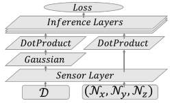
Figure 1 (click to enlarge): General architecture of the Field Probing Neural Network. Note that in addition to the distance transform $D$ used as input, Li et al. also use a normal field as input. In this case, the Gaussian layer is not needed.
The model was trained using stochastic gradient descent on resolution $64 \times 64 \times 64$. Furthermore, while the work was motivated by the low resolution used by other authors, it is unclear why larger resolutions were not evaluated. The presented results are slightly worse than the approach in [2] using multi-view convolutional neural networks. Unfortunately, Li et al. do not discuss possible reasons for this discrepancy.
The implementation is part of Caffe and can be found on GitHub: yanganli/FPNN.
- [1]Z. Wu, S. Song, A. Khosla, F. Yu, L. Zhang, X. Tang, J. Xiao. 3D shapenets: A deep representation for volumetric shapes. CVPR, 2015.
- [2] C. R. Qi, H. Su, M. Nießner, A. Dai, M. Yan, L. Guibas. Volumetric and multi-view cnns for object classification on 3D data. CVPR, 2016.
Qi et al. study how to improve both volumetric convolutional neural networks (CNNs) and multi-view CNNs for 3D shape recognition. In particular, they study the performance gap between these approaches, i.e. volumetric CNNs usually demonstrate inferior performance compared to multi-view CNNs:
"Intuitively, a volumetric representation should encode as much information, if not more, than its multi-view counterpart. However, experiments indicate that multiview CNNs produce superior performance in object classification."
According to Qi et al., this is due to two factors:
- Lower resolution used in volumetric CNNs - usually $30 \times 30 \times 30$ vs. $227 \times 227$ for muli-view CNNs.
- Network architecture differences.
The second argument is motivated by the observation that multi-view CNNs still perform significantly better than volumetric CNNs even in low resolution such as $30 \times 30$. Beneath an extensive evaluation, Qi et al. make the following contributions:
- Introducing auxiliary learning tasks to prevent overfitting of volumetric CNNs.
- Using orientation pooling and data augmentation for volumetric CNNs.
- Introducing anisotropic kernels to probe the volume; several layers with anisotropic kernels implicitly generate multiple "learned" projections of the volume.
They also conducted experiments regarding the influence of resolution on performance, however, they merely experiment with $10 \times 10 \times 10$ and $30 \times 30 \times 30$. As discussed in [1], this is still relatively coarse.
Qi et al. introduce two new network architectures which are both categorized as volumetric CNNs. First, after subsampling the volume, auxiliary tasks to predict the class based on a subvolume are defined. This is done by slicing the obtained volume after the last subsampling/pooling step. Each of these auxiliary tasks tries to predict the class based on roughly $\frac{2}{3}$ of the original volume. As these tasks are considerably more difficult than the original task, this prevents the network from overfitting. The model is illustrated in Figure 1.
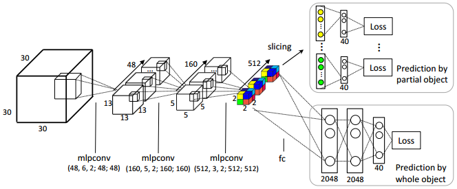
Figure 1 (click to enlarge): Illustration of the network architecture after introducing the auxiliary tasks. Mlpconv corresponds to a network-in-network layer as described in [2]. As can be seen, after subsampling the volume, it is sliced and fed into separate fully-connected networks for prediction.
Second, large anisotropic kernels are used to project the volume onto a single image. This way, instead of using multi-view CNNs where the individual views are pre-computed based on fixed angles, the CNN is able to learn the most appropriate projection for the task. The architecture is illustrated in Figure 2. After the projection, the image is classified using the model described in [2]. Both presented architectures are trained using orientation pooling, aggregating information from different orientations.
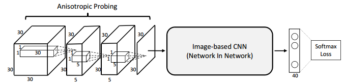
Figure 2 (click to enlarge): Network architecture based on anisotropic probing to learn appropriate projections.
Unfortunately, key details regarding the anisotropic filters and the orientation pooling are omitted. In particular, it is unclear how the anisotropic filters are different from regular filtering in volumes (except for the $1 \times 1$ spatial extend of the filters).
- [1] Yangyan Li, Sören Pirk, Hao Su, Charles Ruizhongtai Qi, Leonidas J. Guibas. FPNN: Field Probing Neural Networks for 3D Data. CoRR, abs/1605.06240.
- [2] Min Lin, Qiang Chen, Shuicheng Yan. Network In Network. CoRR, abs/1312.4400.
Maturana and Scherer, building partly on their work in [1], present VoxNet, a 3D convolutional neural network for object/shape recognition. While the presented model is a simple generalization from 2D convolutional neural networks to the 3-dimensional domain of CAD, LiDAR and RGBD data, the paper presents an excellent introduction and baseline for the topic of 3D object recognition from a deep learning perspective. For example, they discuss three different occupancy grid models used as representation of the data, problems concerning rotational invariance around the z-axis and provide an evaluation and comparison to 3D ShapeNets [2].
As occupancy grid models, they propose to use 3D ray tracing and present the following different representations:
- Binary occupancy grids are based on the discussion by Thrun in [3] where the occupancy of a position $l_{ijk}$ is modeled probabilistically given the sensor measurements $z^1,…,z^t$ as $p(l_{ijk} |z^1,…,z^t)$. The update equation for $l_{ijk}^t$ for measurement $t$ is then given by
$l_{ijk}^t = l_{ijk}^{t - 1} + z^t l_{occ} + (1-z^t)l_{free}$
with $z^t = 1$ if the voxel is hit and $z^t = 0$ if the measurement passes through the voxe. The constants $l_{occ}$ and $l_{free}$ are given by $1.38$ and $-1.38$. - The density grids assigns each voxel a continuous density, as detailed in [4], using the update equations
$\alpha_{ijk}^t = \alpha_{ijk}^{t-1} + z^t$
$\beta_{ijk}^t = \beta_{ijk}^{t - 1} + (1 - z^t)$
and the occupancy estimate$\mu_{ijk}^t = \frac{\alpha_{ijk}^t}{\alpha_{ijk}^t + \beta_{ijk}^t}$
- The hit grid merely counts the number of hits (with a minimum of $1$ hit per voxel). This model discards the difference between free space and unobserved space, but Maturana and Scherer report surprisingly good results using this occupancy grid model.
Based on a occupancy grid as input to the 3d convolutional neural network, they use an architecture consisting of two convolutional layers, a pooling layer and two fully connected layers. The architecture is summarized in Figure 1.
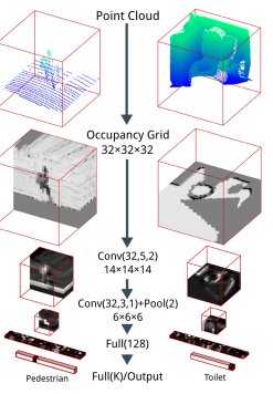
Figure 1 (click to enlarge): Used architecture consisting of two convolutional layers, starting with a resolution of $32^3$, followed by a $2^3$ pooling layer and two fully connected layers.
The training procedure addresses the problem of rotation invariance. The motivation is that it is not trivial to maintain a consistent object orientation relative to the z-axis, while the z-axis itself is assumed to be aligned with the direction of gravity. Therefore, the training set is augmented by several copies of the same model rotated around the z-axis. Experiments show that this approach works well. At testing time, the model is also rotated and the predictions are pooled, resulting in a scheme similar to voting. Additional randomly perturbed as well as mirrored copies further help training.
Experiments are presented on three datasets: a LiDAR dataset, the ModelNet dataset [2] and the NYU Depth Dataset [5]. The approach is compared to the 3D ShapeNet of Wu et al. [26] and shown to outperform 3D ShapeNet with considerably less parameters on all tasks except the cross-domain task where the model is trained on a different dataset than it is evaluated on.
- [1] D. Maturana, S. Scherer. 3D convolutional neural networks for landing zone detection from lidar. ICRA, 2015.
- [2] Z. Wu, S. Song, A. Khosla, F. Yu, L. Zhang, X. Tang, J. Xiao. 3d shapenets: A deep representation for volumetric shape modeling. CVPR, 2015.
- [3] S. Thrun. Learning occupancy grid maps with forward sensor models. Auton. Robots, 2003.
- [4] D. Hähnel, D. Schulz, W. Burgard. Map building with mobile robots in populated environments. IROS, 2002
- [5] P. K. Nathan Silberman, Derek Hoiem, R. Fergus. Indoorsegmentation and support inference from rgbd images. ECCV, 2012.
Results of some of these approaches in the "Large-Scale 3D Shape Retrieval from ShapeNet Core55" 2016 can be found in the corresponding report:
Dai et al. use a 3D convolutional neural network architecture called 3D-Encoder-Predictor Network for shape completion. Figure 1 illustrates the high-level pipeline. The first step consists of two networks which are combined in the framework of their 3D Encoder-Preodictor Network as illustrated in Figure 2. The input is a two channel volume encoding the signed truncated distance function (STDF) and the output is only a distance function (DF). Nearest neighbors of the output shape (in resolution $32^3$) are searched utilizing features taken from a 3D classification network following []. Finally, the output volume and the nearest neighbor shapes are used to produce a higher-resolution mesh ($128^3$), see the paper for details.
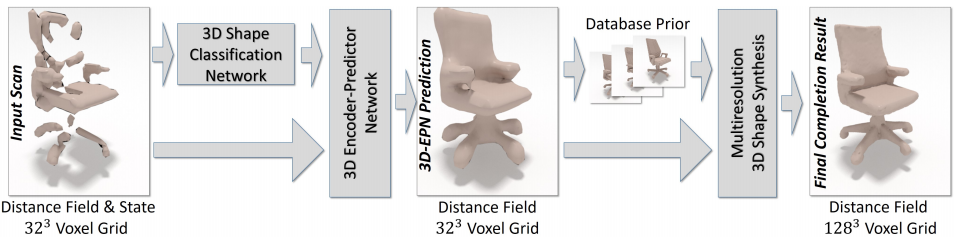
Figure 1 (click to enlarge): High-level illustration of the proposed approach as described in the text.
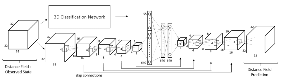
Figure 2 (click to enlarge): The network architecture used for shape completion.
- [] C. R. Qi, H. Su, M. Nießner, A. Dai, M. Yan, and L. Guibas. Volumetric and multi-view cnns for object classification on 3D data. In Proc. Computer Vision and Pattern Recognition (CVPR), 2016.
The following two references propose neural networks on point sets:
Garcia-Garcia et al. present several experiments conducted using VoxNet [] on density occupancy grids for 3D shape classification. The used network architecture is shown in Figure 1 – they introduce a so-called PC Data Layer which converts a point cloud into a density grid, i.e. a voxel grid where each voxel represents the number of points within the voxel. On the ModelNet dataset [], they convert the given meshes into point clouds using ray tracing. An example of their representation is shown in Figure 2. Except for the change in representation, they do not introduce changes to the architecture.
![]()
Figure 1 (click to enlarge): Used architecture, where the PC Data Layer is described in the text. The parameters, i.e. $300$ and $5$ correspond to a voxel grid of $60^3$, i.e. $300^3$ units with voxel size $5^3$.

Figure 2 (click to enlarge): Illustration of the used representation. From left to right: original mesh, point cloud obtained by ray tracing and density voxel grid fed into the 3D convolutional neural network.
Interestingly, they report that deeper networks are not able to increase performance. They attribute this fact to severe over-fitting and the highly unbalanced ModelNet10. Unfortunately, they only experiment with two different architectures, where the second one adds only one additional convolutional layer to the architecture depicted in Figure 1. Additionally, they do not present any experiments to overcome these difficulties.
- [] D. Maturana and S. Scherer. Voxnet: A 3d convolutional neural network for real-time object recognition. IROS, 2015.
- [] Z. Wu, S. Song, A. Khosla, F. Yu, L. Zhang, X. Tang, and J. Xiao, 3d shapenets: A deep representation for volumetric shapes. in Proceedings of the IEEE Conference on Computer Vision and Pattern Recognition, 2015, pp. 1912–1920.
Applications in medical imaging:
Milletari et al. discuss volumetric, fully convolutional neural networks for medical image segmentation. Concretely, they use the architecture depicted in Figure 1 to segment MRI volumes. Due to the limited training set size, the data was augmented by random deformations and intensity adaptations. The network architecture combines a compression and a decompression part. Both parts consist of several stages, each stage comprising several convolutional layers, followed by adding the input (i.e. to learn the residual) and a downsampling stage (which is implemented by strided convolution in contrast to max pooling). In order to cope with the inbalanced label distribution in the volumes, they propose the dice loss:
$D = \frac{2\sum_i^N p_i g_i}{\sum_i^N p_i^2 + \sum_i^N g_i^2}$
where $N$ is the number of voxels, $p_i$ the foreground probability of the prediction and $q_i$ the foreground probability of the ground truth segmentation. As discussed in the paper, the dice loss is differentiable and allows training without assigning weights to the different classes. They provide experimental results on the PROMISE 2012 challenge dataset, see the paper.
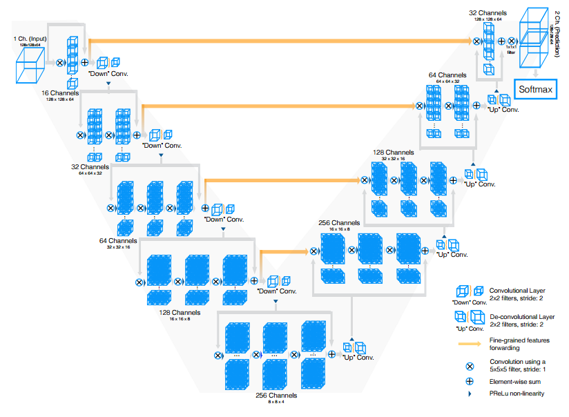
Figure 1 (click to enlarge): Illustration of the used network architecture consisting of a compression path (left) and a decompression path (right).
Cicek et al. present a 3D convolutional network architecture for volumetric segmentation in the biomedical domain from sparse annotations. In particular, they propose the architecture shown in Figure 1, closely related to earlier work [1]. The network combines a decode stage, consisting of several convolutional and pooling layers, with a decoder part consisting of a series of convolutional and up-convolutional layers. Key to their model is that the loss function disregards voxels labeled as "unlabeled". Therefore, the network can be trained using volumes where only a few slices are densely labeled. They further utilize heavy data augmentation including rotations, gray value augmentation and smooth deformations.

Figure 1 (click to enlarge): Illustration of the network architecture.
- [1] O. Ronneberger, P. Fischer, T. Brox. U-net: Convolutional networks for biomedical image segmentation. MICCAI, 2015.
Dou et al. propose an efficient approach to cerebral microbleeds detection in 3D MR volumes/images using 3D convolutional networks. Cerebral microbleeds are small areas of blood products within normal brain tissues. They have been identified as important symptom for diagnosing cerebrovascular diseases. However, manual detection is error prone, motivating the use of computer vision based systems for detection. An example can be found in Figure 1.
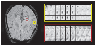
Figure 1 (click to enlarge): Illustration of an MR scan and a cerebral microbleed (in yellow) and a mimic (in red).
The proposed approach is a two-stage system consisting of a fully convolutional detection proposal system, and a discriminator to reduce false positives. In both cases, convolutional neural networks are generalized to 3D data in the straight-forward manner (by using 3D kernels for convolutions). The used architectures of both models are summarized in Figure 2, where $M$ denotes a max pooling layer, $C$ a convolutional layer and $FC$ a fully connected layer. For the fully convolutional network, the fully connected layers are reinterpreted as convolutional layers. Thus, the network can be trained on positive/negative crops of the 3D data and during testing be applied to full 3D volumes to produce probability volumes. After non-maximum suppression and thresholding, the probability volume is used to extract detection proposals. The discriminator is a general 3D convolutional neural network trained on crops including false positives obtained from the fully convolutional network. The full system and training procedure are illustrated in Figure 3.
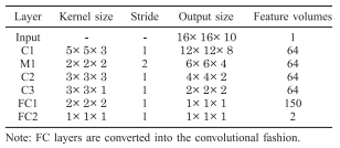
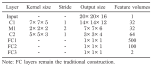
Figure 2 (click to enlarge): Network architectures for the fully convolutional detection proposal network (left) and the discriminator network (right).
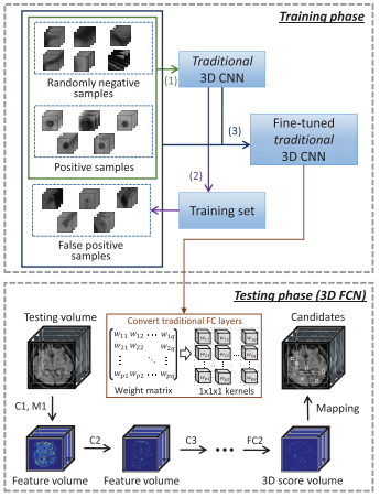
Figure 3 (click to enlarge): Illustration of training and testing of the full system.
On a newly created dataset of MR images, they show promising results (as far as I can judge) and demonstrate superiority regarding hand-crafted features, combined with random forests or SVMs. They also evaluate the detection proposal network separately to show that the number of false positives and false negatives is reduced compared to other approaches.
Chen et al. propose to apply residual units [1,2] to segmentation of brain scans. As the scans represent volumetric information, a 3D convolutional neural network is used. The network is summarized in Figure 1.
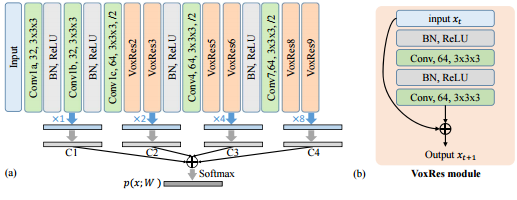
Figure 1 (click to enlarge): Illustration of the employed architecture.
Additionally, Chen et al. use the proposed architecture in an auto-context fashion. This means that one VoxResNet is trained on the training set. Based on the probability maps produced by this VoxResNets, another VoxResNet is trained taking these probability maps as additional "context"-input.
- [1] K. He, X. Zhang, S. Ren, J. Sun. Deep residual learning for image recognition. CoRR, 2015.
- [2] K. He, X. Zhang, S. Ren, J. Sun. Identity mappings in deep residual networks. CoRR, 2016.
Object detection on various datasets:
Li discusses a simple 3D fully convolutional network for 3D object detections on KITTI []. The approach is considerably simple and the used architecture is summarized in Figure 1. A fully convolutional network naturally extends to the 3D domain, operating on an occupancy grid where each voxel is either occupied (equals $1$) or not. The output of the network is an objectness score per pixel (although the output is subsampled by $\frac{1}{4}^3$ compared to the input) and a bounding box per pixel. At testing time, the bounding boxes of positive object pixels are clustered to get a prediction (which corresponds to implicit non-maximum suppression). The bounding boxes are encoded as the corresponding corners in 3D. The model is evaluated on the KITTI dataset; without discussing the numbers, Figure 2 shows qualitative results.
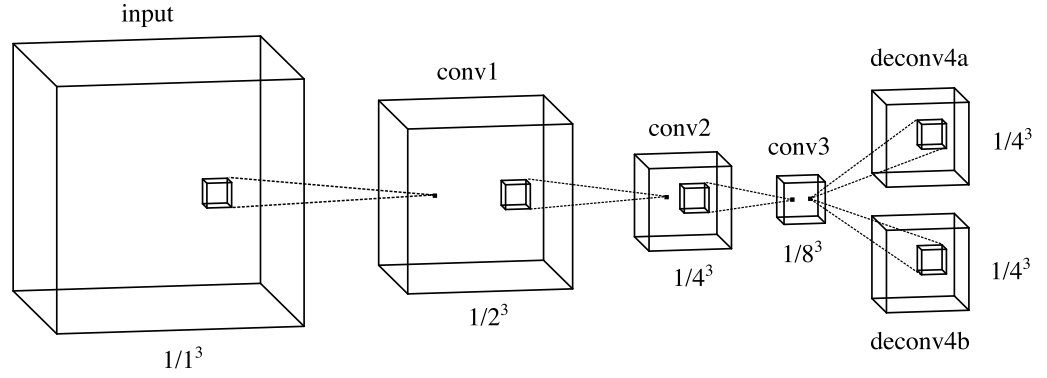
Figure 1 (click to enlarge): Illustration of the simple network used for object detection. Unfortunately, details on the number of channels and filter sizes are missing.
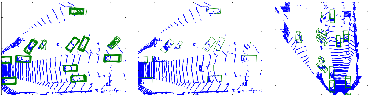
Figure 2 (click to enlarge): Qualitative results demonstrating the objectness and bounding box predictions (left), the detections after clustering (middle) and the 3D bounding box predictions (right).
- [] Andreas Geiger, Philip Lenz, and Raquel Urtasun. Are we ready for autonomous driving? the KITTI vision benchmark suite. Proceedings of the IEEE Computer Society Conference on Computer Vision and Pattern Recognition, pages 3354–3361, 2012.
Chen et al. propose a multiv-view convolutional neural network for 3D object detection – called Multi-View 3D Object Detection Network (MV3D). While the task is to predict 3D bounding boxes, the convolutional neural network operators on 2D projections of the LiDAR information. This allows the network to fuse LiDAR information and RGB information in a “deep fashion”.
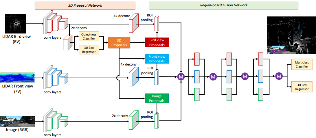
Figure 1 (click to enlarge): Network architecture comprising the proposal network and the fusion network as well as illustrating the used input data.
The given LiDAR data is projected in two ways. First in bird’s view, and in front view. In both cases, different channels are hand-crafted. Together with the RGB information, the information is purely 2D. Chen et al. then discuss a 3D Proposal Network that operates purely on the bird’s eye and a region-based Fusion Network. Both are illustrated in Figure 1. While the general structure follows related work (e.g. R-CNN) in that the proposal network predicts objectness and bounding boxes and Region-of-Interest Pooling is then used to apply the classifier on top, a key contribution is the fusion network. Instead of fusing the different inputs (i.e. LiDAR and RGB) before the network (early fusion) or at the end of the network (late fusion), they propose to fuse the information in every step using element-wise mean operations (see Figure 1).

Figure 2 (click to enlarge): Qualitative results comparing 3DOP [] (left), VeloFCN [] (middle) and the proposed approach (right).
The presented experiments are based on VGG16 [] and the KITTI dataset []. Qualitative results are shown in Figure 2. In an ablation study they demonstrate the advantage of using their fusion model and additionally adding auxiliary losses as regularization.
- [] X. Chen, K. Kundu, Y. Zhu, A. Berneshawi, H. Ma, S. Fidler, and R. Urtasun. 3d object proposals for accurate object class detection. In NIPS, 2015.
- A. Geiger, P. Lenz, and R. Urtasun. Are we ready for autonomous driving? the kitti vision benchmark suite. In CVPR, 2012.
- [] B. Li, T. Zhang, and T. Xia. Vehicle detection from 3d lidar using fully convolutional network. In Robotics: Science and Systems, 2016.
- [] K. Simonyan and A. Zisserman. Very deep convolutional networks for large-scale image recognition. In arXiv:1409.1556, 2014.
Song and Xiao propose to use 3D convolutional neural networks for 3D object detection in RGB-D images as provided by the NYU Depth Dataset v2 [1] or the SUN RGBD dataset [2]. The approach is splitted into an object recognition network jointly using 3D shape and 2D color features, and a region proposal network.
The region proposal network is applied to bounding boxes of varying shape and orientation sampled across the whole 3D scene and outputs an objectness score. It is also supposed to perform bounding box regression (i.e. predict the difference between the input bounding box size and the object bounding box size). To this end, the point cloud is voxelized using the directed Truncated Signed Distance Function. This means, that the space is divided into voxels and each voxel is represented by a vector encoding the shortest direction to the surface obtained from the RGB-D image used as input. The 3D scene is aligned with the direction of gravity and sampled with a grid size of $0.025$ meters resulting in a voxel grid of size $208 \times 208 \times 100$. The main directions of the scene are estimated using RANSAC (based on the Manhatten world assumption) and all objects are assumed to be aligned with these directions. At each anchor position of the sliding window based approach, the network predicts $19$ different scores corresponding to bounding boxes illustrated in Figure 1. Additionally, the network operates at different scales — for larger scales an additional pooling layer is used to increase the receptive field. Additionally, bounding box regression is performed by predicting the deviation from the predicted, fixed bounding box as in Figure 1. To this end, a multi-task loss is used where bounding box regression is trained using a smooth $L_1$ loss. The overall architecture is illustrated in Figure 2. For training, samples are labeled according to their 3D intersection over union score and each batch contains the positive and negative samples for a specific image. See the paper for the details.
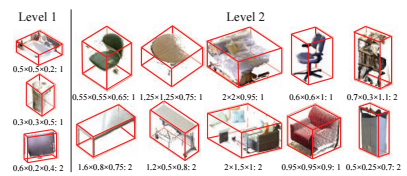
Figure 1 (click to enlarge): List of the used anchor types, i.e. bounding box shapes. The subtitles of the boxes describe the 3D extends as well as the number of orientations used.
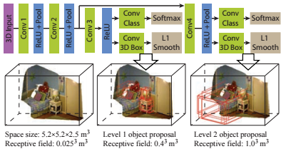
Figure 2 (click to enlarge): Illustration of the network architecture used for the region proposal network.
The object recognition network takes the proposals from the region proposal networks and divides the corresponding space into $30 \times 30 \times 30$ voxels (after padding). The voxel grid is used for classification based on the shape. However, Song and Xiao additionally use color information. Therefore, the points in the point cloud contained within the bounding box are backprojected to the image plane and the VGGnet [3] (pre-trained on ImageNet) is used to compute color features which are then fed into the overall object recognition network. This structure is illustrated in Figure 3.
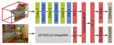
Figure 3 (click to enlarge): Illustration of the network architecture used for the object recognition network. The network combines learned features from the 3D shape obtained from a $30 \times 30 \times 30$ voxel grid, and color features obtained from VGGnet [3].
The results look promising, outperforming their prior work called Sliding Shapes [4] by a significant margin. Furthermore, they discuss the region proposal network and show a significant performance boost in contrast to a 3D selective search algorithm (see the paper for details). Qualitative results, and a comparison with Sliding Shapes, can be found in Figure 4.
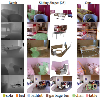
Figure 4 (click to enlarge): Qualitative results and comparison with Sliding Shapes.
- [1] N. Silberman, D. Hoiem, P. Kohli, R. Fergus. Indoor segmentation and support inference from RGBD images. ECCV, 2012.
- [2] S. Song, S. Lichtenberg, J. Xiao. SUN RGB-D: A RGBD scene understanding benchmark suite. CVPR, 2015.
- [3] K. Simonyan, A. Zisserman. Very deep convolutional networks for large-scale image recognition. CoRR, 2014.
- [4] S. Song, J. Xiao. Sliding Shapes for 3D object detection in depth images. ECCV, 2014.
Li et al. perform vehicle detection in 3D Lidar data using fully convolutional networks. To this end, they propose to run 2D fully connected convolutional networks on point maps, i.e. backprojections of the 3D Lidar data to the image plane. An example of a point map is shown in Figure 1.
Figure 1 (click to enlarge): Illustration of the used point map created from the 3D Lidar data.
The network architecture strongly mirrors the architectures used in [1] and [2] and is shown in Figure 2. The convolutional layers conv1 to conv3 are followed by pooling layers to subsample the feature maps. Note that conv1 subsamples the input by 4 pixels horizontally and 2 pixels vertically. This is because by construction of the point map is denser in the horizontal direction. The subsampled feature maps are then combined and upsampled to predict two outputs: an objectness score per point, and a 3D bounding box per point (bounding box map and objectness map in Figure 2).
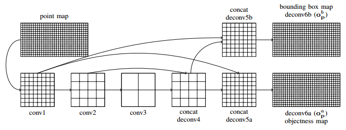
Figure 2 (click to enlarge): Illustration of the used architecture.
Objectness is represented by a 2-unit Softmax output, trained using negative log-likelihood. The bounding boxes are represented by 8 corner points which are predicted simultaneously. For details on the corner point representation, see the paper. To balance positive and negative sample points (i.e. vehicle and non-vehicle points), negative points are re-weighted. Similarly, to avoid a bias towards close vehicles, positive samples closer to the Velodyne sensor are re-weighted, as well. Training is performed jointly minimizing the negative log-likelihood and the Euclidean distance of bounding boxes. During training, samples are transformed using random transformations in 3D close to the identity transformation. The approach is evaluated on the KITTI test set and shows promising results, among others compared to Vote3D [3].
- [1] L. Huang, Y. Yang, Y. Deng, Y. Yu. DenseBox: Unifying Landmark Localization with End to End Object Detection. CoRR, 2015.
- [2] J. Long, E. Shelhamer, T. Darrell. Fully convolutional networks for semantic segmentation. CoRR, 2014.
- [3] D. Zeng Wang, I. Posner. Voting for voting in online point cloud object detection. Robotics: Science and Systems, 2015.
Some papers discussing efficient training (in particular efficient convolutions in sparse occupancy volumes) or sparse convolutional neural networks:
Notchenko present PySparseConvNet, a Python interface for SparseConvNet as introduced by Graham in []. They further conduct several experiments for shape retrieval and shape classification also investigating the influence of the resolution, see the paper for details.
- [] B. Graham. Spatially-sparse convolutional neural networks. arXiv preprint arXiv:1409.6070, 2014.
Engelcke et al. use sparse 3D convolutional neural networks for 3D object detection on the KITTI [1] benchmark. Following earlier work [2], they use sparse convolutions to implement 3D convolutions on sparse 3D data. To this end, they convert the input point cloud into an occupancy grid where each grid cells holds statistics about the underlying points. As this occupancy grid is very sparse, performing regular 3D convolutions is computationally prohibitive. Instead of evaluating the kernel at every location in the grid, they flip the kernel, lay it over every non-zero voxel such that these can "cast votes" for neighboring voxels. This scheme is illustrated in Figure 1. Overall, this scheme highly reduces the computational effort needed for 3D convolutions.

Figure 1 (click to enlarge): Illustration of the voting scheme used to efficiently compute convolutions in sparse data. The example shows the voting scheme applied to sparse 2D grids. Instead of applying the kernel (center left) to every position in the grid, resulting in many zero multiplications, the kernel is flipped (center right) and applied to every non-zero position in the grid (indicated by the two green rectangles, right). The kernel is then used to cast votes regarding the new values of neighboring voxels.
For object detection on KITTI, they use a fixed size bounding box for each category (e.g. pedestrian, vehicle, ciclyst etc.). For each category, a binary classifier is used — represented by comparably shallow 3D convolutional networks as illustrated in Figure 2. Each sparse convolutional layer is followed by rectified linear units in order to preserve sparsity. Furthermore, biases used in the convolutional layers are constrained to be negative. Training is done using the hinge loss, including weight decay and a $L_1$ regularizer for sparsity. The model is trained on an augmented set of positive and negative examples by randomly rotating and translating them. Every no and then, hard negatives are mined and added to the training set.
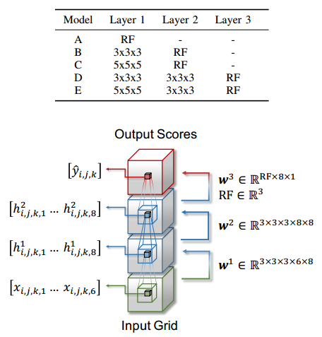
Figure 2 (click to enlarge): Summary of the evaluated models. They use different models for different classes, however, overall the models are comparably shallow.
The performance is compared to other state-of-the-art methods, including their earlier work [2], on the KITTI test set and demonstrates significantly improved accuracies.
- [1] A. Geiger, P. Lenz, R. Urtasun. Are we ready for autonomous driving? the KITTI vision benchmark suite CVPR, 2012.
- [2] D. Z. Wang, I. Posner. Voting for Voting in Online Point Cloud Object Detection. Robotics Science and Systems, 2015.
Graham generalizes sparse convolutional neural networks previously considered in [1] to 3D data. His approach is twofold:
- A square grid in 2D can be replaced by a triangular grid. Similarly, in 3D, a cubic grid can be replaced by a tetrahedral grid, as illustrated in Figure 1. This scheme can be applied to convolutions and pooling and offers to reduce the complexity.
- On sparse input data, convolutions only need to consider non-zero entries. Graham, therefore, uses hashmaps to efficiently store and identify non-zero entries in the cubic/tetrahedral grid to speed up convolutions.
Graham conducts several experiments meant as proof of concept how these two techniques can be used to speed up 3D convolutional networks, see the paper.

Figure 1 (click to enlarge): Illustration of different grid representations used by Graham.
The idea with a tetrahedral grid seems interesting, but concerning the speeded up convolutions, the approach by Engelcke et al. [2] seems more elegant.
- [1] B. Graham. Spatially-sparse convolutional neural networks. 2014.
- [2] M. Engelcke, D. Rao, D. Z. Wang, C. H. Tong, I. Posner. Vote3Deep: Fast Object Detection in 3D Point Clouds Using Efficient Convolutional Neural Networks. CoRR, 2016.
Other applications:
Yumer and Mitra use 3D convolutional neural networks to predict semantic shape deformations. In particular, they consider shoes, cars, chairs and airplanes and deformations such as "comfy" for shoes or "sporty" for cars. The used network architecture corresponds to an encoder decoder scheme as illustrated in Figure 1. Results are shown in Figure 2.
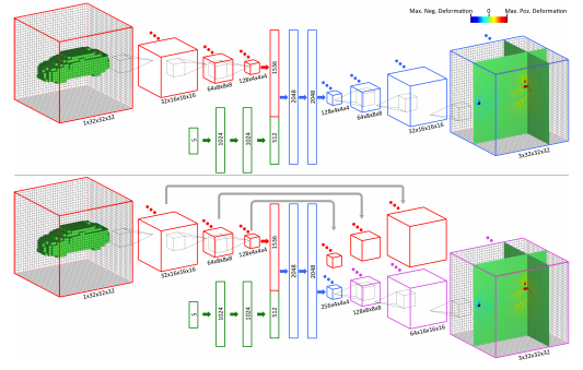
Figure 1 (click to enlarge): The proposed network architectures to predict semantic shape deformations.
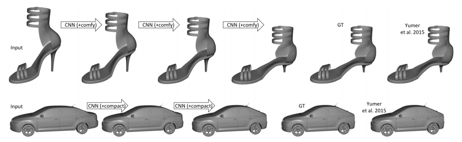
Figure 2 (click to enlarge): Qualitative results.
Huang and You use simple 3D convolutional networks for point cloud labeling. Given a big point cloud, e.g. consisting of a part of Ottawa, they extract individual point clouds by moving a center point through the point cloud and extracting a cubic bounding box with defined radius. The extracted point cloud is transformed to a voxelized occupancy grid used as input. The labels are inferred using a voting scheme for each voxel (as multiple labels can be present in each voxel). They claim to use $8000$ cells as input, which would correspond to $20 \times 20 \times 20$. This is, indeed, rather small, as they claim that 3D convolutional networks quickly reach the memory limit.
The used network is rather simple and supposed to perform per-pixel semantic segmentation. Motivated by LeNet [1], the network consists of two 3D convolutional layers (where the convolutional layer is extended to 3D in a straight-forward way) and two 3D pooling layers, followed by a fully connected layer. This is illustrated in Figure 1. They present qualitative results in Figure 2.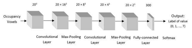
Figure 1 (click to enlarge): Illustration of the used network architecture.
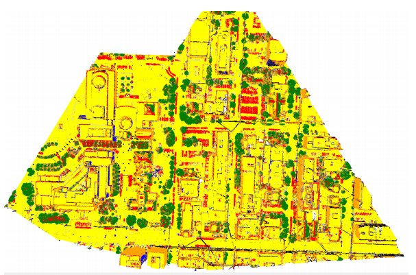
Figure 2: Qualitative results.
- [1] Y. LeCun, L. Bottou, Y. Bengio, P. Haffner. Gradient-based learning applied to document recognition. Proceedings of the IEEE, 1998.
Maturana and Scherer (also see [1] for their follow up work) tackle the problem of safe landing zone recognition using 3d convolutional neural networks. While the system itself merely generalizes convolutional neural networks to 3d volumes, trained on occupancy maps as input, Maturana and Scherer also focus on computing the occupancy maps in an efficient and reasonable way — see the discussion in [2] for details — and on generating appropriate synthetic dataset to evaluate the system. On a high level (also see my notes on [1] for details), the 3d convolutional neural nework combines one or two convolutional layers including max pooling and ReLU activations with two fully connected layers. Training is done on augmented training sets including rotated input for rotational invariance.
- [1] Daniel Maturana, Sebastian Scherer. VoxNet: A 3D Convolutional Neural Network for real-time object recognition. IROS, 2015.
- [2] G. D. Tipaldi, K. O. Arras. FLIRT - interest regions for 2D range data. ICRA, 2010.
Future Readings
There is quite some interest in 3D convolutional neural networks — or deep learning in 3D in general. So there are several papers that are still on my reading list:
- Evangelos Kalogerakis, Melinos Averkiou, Subhransu Maji, Siddhartha Chaudhuri. 3D Shape Segmentation with Projective Convolutional Networks. CoRR abs/1612.02808 (2016).
- Xinchen Yan, Jimei Yang, Ersin Yumer, Yijie Guo, Honglak Lee. Perspective Transformer Nets: Learning Single-View 3D Object Reconstruction without 3D Supervision. NIPS 2016: 1696-1704.
- Maxim Tatarchenko, Alexey Dosovitskiy, Thomas Brox. Octree Generating Networks: Efficient Convolutional Architectures for High-resolution 3D Outputs. CoRR abs/1703.09438 (2017).
- Min Liu, Yifei Shi, Lintao Zheng, Yueshan Xiong, Kai Xu. Volumetric spatial transformer network for object recognition. SIGGRAPH Asia Posters 2016: 38.
- Gernot Riegler, Ali Osman Ulusoy, Horst Bischof, Andreas Geiger. OctNetFusion: Learning Depth Fusion from Data. CoRR abs/1704.01047 (2017).
- Peng-Shuai Wang, Yang Liu, Yu-Xiao Guo, Chun-Yu Sun, and Xin Tong. 2017. O-CNN: Octree-based Convolutional Neural Networks for 3D Shape Analysis. ACM Trans. Graph. (SIGGRAPH) 36, 4 (July 2017).
- Maxim Tatarchenko, Alexey Dosovitskiy, Thomas Brox. Octree Generating Networks: Efficient Convolutional Architectures for High-resolution 3D Outputs. CoRR abs/1703.09438 (2017).
References
- [] Xiaozhi Chen, Huimin Ma, Ji Wan, Bo Li, Tian Xia. Multi-View 3D Object Detection Network for Autonomous Driving. CoRR abs/1611.07759 (2016).
- [] Alberto Garcia-Garcia, Francisco Gomez-Donoso, José García Rodríguez, Sergio Orts-Escolano, Miguel Cazorla, Jorge Azorín López .PointNet: A 3D Convolutional Neural Network for real-time object class recognition. IJCNN 2016: 1578-1584.
- [] Rohit Girdhar, David F. Fouhey, Mikel Rodriguez, Abhinav Gupta. Learning a Predictable and Generative Vector Representation for Objects. ECCV (6) 2016: 484-499.
- [] Angela Dai, Charles Ruizhongtai Qi, Matthias Nießner. Shape Completion using 3D-Encoder-Predictor CNNs and Shape Synthesis. CoRR abs/1612.00101 (2016).
- [] Abhishek Sharma, Oliver Grau, Mario Fritz. VConv-DAE: Deep Volumetric Shape Learning Without Object Labels. ECCV Workshops (3) 2016: 236-250.
- [] Fausto Milletari, Nassir Navab, Seyed-Ahmad Ahmadi. V-Net: Fully Convolutional Neural Networks for Volumetric Medical Image Segmentation. 3DV 2016: 565-571.
- [] Vishakh Hegde, Reza Zadeh. FusionNet: 3D Object Classification Using Multiple Data Representations. CoRR abs/1607.05695 (2016).
- [] Hao Chen, Qi Dou, Lequan Yu, Pheng-Ann Heng. VoxResNet: Deep Voxelwise Residual Networks for Volumetric Brain Segmentation. CoRR abs/1608.05895 (2016).
- [] Qi Dou, Hao Chen, Lequan Yu, Lei Zhao, Jing Qin, Defeng Wang, Vincent C. T. Mok, Lin Shi, Pheng-Ann Heng. Automatic Detection of Cerebral Microbleeds From MR Images via 3D Convolutional Neural Networks. IEEE Trans. Med. Imaging 35(5): 1182-1195 (2016).
- [] Özgün Çiçek, Ahmed Abdulkadir, Soeren S. Lienkamp, Thomas Brox, Olaf Ronneberger. 3D U-Net: Learning Dense Volumetric Segmentation from Sparse Annotation. MICCAI (2) 2016: 424-432.
- [] Ben Graham. Sparse 3D convolutional neural networks. BMVC 2015: 150.1-150.9.
- [] Bo Li, Tianlei Zhang, Tian Xia. Vehicle Detection from 3D Lidar Using Fully Convolutional Network. Robotics: Science and Systems 2016.
- [] Nima Sedaghat, Mohammadreza Zolfaghari, Thomas Brox. Orientation-boosted Voxel Nets for 3D Object Recognition. CoRR abs/1604.03351 (2016).
- [] Shuran Song, Jianxiong Xiao. Deep Sliding Shapes for Amodal 3D Object Detection in RGB-D Images. CVPR 2016: 808-816.
- [] André Brock, Theodore Lim, James M. Ritchie, Nick Weston. Generative and Discriminative Voxel Modeling with Convolutional Neural Networks. CoRR abs/1608.04236 (2016).
- [] Martin Engelcke, Dushyant Rao, Dominic Zeng Wang, Chi Hay Tong, Ingmar Posner. Vote3Deep: Fast Object Detection in 3D Point Clouds Using Efficient Convolutional Neural Networks. CoRR abs/1609.06666 (2016).
- [] Yangyan Li, Sören Pirk, Hao Su, Charles Ruizhongtai Qi, Leonidas J. Guibas. FPNN: Field Probing Neural Networks for 3D Data. NIPS 2016: 307-315.
- [] Charles Ruizhongtai Qi, Hao Su, Matthias Nießner, Angela Dai, Mengyuan Yan, Leonidas J. Guibas. Volumetric and Multi-view CNNs for Object Classification on 3D Data. CVPR 2016: 5648-5656
- [] Zhirong Wu, Shuran Song, Aditya Khosla, Fisher Yu, Linguang Zhang, Xiaoou Tang, Jianxiong Xiao. 3D ShapeNets: A deep representation for volumetric shapes. CVPR 2015: 1912-1920.
- [] Daniel Maturana, Sebastian Scherer. VoxNet: A 3D Convolutional Neural Network for real-time object recognition. IROS 2015: 922-928
- [] Hang Su, Subhransu Maji, Evangelos Kalogerakis, Erik G. Learned-Miller. Multi-view Convolutional Neural Networks for 3D Shape Recognition. ICCV 2015: 945-953.
- [] Jiajun Wu, Chengkai Zhang, Tianfan Xue, Bill Freeman, Josh Tenenbaum. Learning a Probabilistic Latent Space of Object Shapes via 3D Generative-Adversarial Modeling. NIPS 2016: 82-90
- [] Shuiwang Ji, Wei Xu, Ming Yang, Kai Yu. 3D Convolutional Neural Networks for Human Action Recognition. IEEE Trans. Pattern Anal. Mach. Intell. 35(1): 221-231 (2013).
- [] Gernot Riegler, Ali Osman Ulusoy, Andreas Geiger. OctNet: Learning Deep 3D Representations at High Resolutions. CoRR abs/1611.05009 (2016).